3 Kalman Filter

This chapter is the foundation for understanding Kalman filter and its mathematics.

The main reference for this chapter is Simon (2006).

Some key points on Kalman filter are

Kalman filter operates by propagating the mean and covariance of the state through time (previous chapter).
Mean of the state at given time is the Kalman filter estimate of the state. Covariance of the state is the covariance of the Kalman filter state estimate.
The mean and covariance of the state is updated every time when new measurement data is received. This is raised from the recursive least squares seen in chapter 1.

3.1 Discrete Kalman filter derivation

Let a linear discrete-time system is given as

\[ \begin{align} \mathbf{x}_k &= \mathbf{F}_{k-1}\mathbf{x}_{k-1} + \mathbf{G}_{k-1}\mathbf{u}_{k-1} + \mathbf{w}_{k-1} \\ \mathbf{y}_k &= \mathbf{H}_k \mathbf{x}_k + \mathbf{v}_k \end{align} \tag{3.1}\]

The noises \(\mathbf{w}_k,\mathbf{v}_k\) are assumed to be zero-mean, white, uncorrelated and have known covariance matrices \(\mathbf{Q}_k,\mathbf{R}_k\) respectively. Thus,

\[ \begin{align} \mathbf{w}_k &\sim (\mathbf{0},\mathbf{Q}_k) \\ \mathbf{v}_k &\sim (\mathbf{0},\mathbf{R}_k) \\ E(\mathbf{w}_k\mathbf{w}_j^T) &= \mathbf{Q}_k\delta_{k-j}\\ E(\mathbf{v}_k\mathbf{v}_j^T) &= \mathbf{R}_k\delta_{k-j}\\ E(\mathbf{w}_k\mathbf{v}_j^T) &= 0 \end{align} \tag{3.2}\]

Now, there are four kinds of estimations

Posteriori estimate,
Priori estimate,
Smoothed estimate and
Predicted estimate

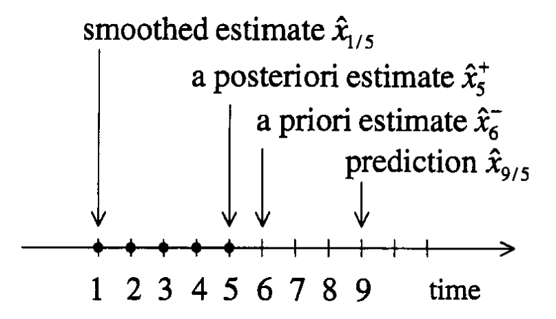
Posteriori estimate is the estimate of \(\hat{\mathbf{x}}_k\) after processing the measurement \(\mathbf{y}_k\) at the k^th timestep, represented by \(\hat{\mathbf{x}}^+_k\).

Priori estimate is the estimate of \(\hat{\mathbf{x}}_k\) before processing the measurement \(\mathbf{y}_k\) at the k^th timestep, represented by \(\hat{\mathbf{x}}^-_k\).

Smoothed estimate is the estimate of \(\hat{\mathbf{x}}_k\) obtained after processing the past, present and future measurement data, represented by \(\hat{\mathbf{x}}_{k|k+N}\) where \(N\) is a positive non-zero number.

Predicted estimate is the estimate of \(\hat{\mathbf{x}}_k\) obtained after processing the measurement data from past till on or before second last measurement data. In other words, it is the estimate of \(\hat{\mathbf{x}}_k\) more than one time step ahead of the available measurements. It is represented as \(\hat{\mathbf{x}}_{k|k-M}\).

The following figure represents visually the above estimate types.

Now, using the above representation, the mean state estimate equation Eq. 2.2 can be written as

\[ \hat{\mathbf{x}}_k^- = \mathbf{F}_{k-1}\mathbf{x}_{k-1}^+ + \mathbf{G}_{k-1}\mathbf{u}_{k-1} . \tag{3.3}\]

Similarly, the state covariance estimate equation Eq. 2.3 cab be written as

\[ \mathbf{P}_k^- = \mathbf{F}_{k-1}\mathbf{P}_{k-1}^+\mathbf{F}_{k-1}^T+\mathbf{Q}_{k-1} . \tag{3.4}\]

And, finally the update equations given in Section 1.3.3 is rewritten as

\[ \begin{align} \mathbf{K}_k &= \mathbf{P}^-_{k}\mathbf{H}_k^T\left(\mathbf{H}_k\mathbf{P}^-_{k}\mathbf{H}_k^T+\mathbf{R}_k\right)^{-1} \\ &= \mathbf{P}^+_k\mathbf{H}_k^T\mathbf{R}_k^{-1} \\ \hat{\mathbf{x}}^+_k &= \hat{\mathbf{x}}^-_{k} + \mathbf{K}_k\left(\mathbf{y}_k - \mathbf{H}_k\hat{\mathbf{x}}^-_{k}\right) \\ \mathbf{P}^+_k &= \left(\mathbf{I}-\mathbf{K}_k\mathbf{H}_k\right)\mathbf{P}^-_{k}\left(\mathbf{I}-\mathbf{K}_k\mathbf{H}_k\right)^T + \mathbf{K}_k\mathbf{R}_k\mathbf{K}_k^T \\ &= \left[\left(\mathbf{P}^-\right)_{k}^{-1} + \mathbf{H}_k^T\mathbf{R}_k^{-1}\mathbf{H}_k\right]^{-1} \\ &= \left(\mathbf{I} - \mathbf{K}_k\mathbf{H}_k\right)\mathbf{P}_{k}^- \end{align} \tag{3.5}\]

In Eq. 3.5, the first expression for \(\mathbf{P}_k^+\) is called Joseph stabilized equation. It guarantees that \(\mathbf{P}_k^+\) will always be symmetric positive definite, as long as \(\mathbf{P}_k^-\) is symmetric and positive definite. Third expression is computationally simpler but does not guarantee symmetry and positive definiteness. The second form is rarely implemented but will be used in later chapters.

In Eq. 3.5, if second expression for \(\mathbf{K}_k\) is used, then the second expression for \(\mathbf{P}_k^+\) is to be used as it is independent of \(\mathbf{K}_k\) but the converse is true.

Note that if \(\mathbf{x}_k\) is constant, then \(\mathbf{F}_k = \mathbf{I}\), \(\mathbf{Q}_k=0\) and \(\mathbf{u}_k=0\). It reduces the Eq. 3.5 to the recursive least squares algorithm given in Section 1.3.3.

An important practical aspect of Kalman filer is that, in Eq. 3.5 the \(\mathbf{P}_k^-,\mathbf{K}_k,\mathbf{P}_k^+\) is independent of measurements. So, they can be computed offline and used for online estimation thereby saving resources. Only \(\hat{\mathbf{x}}_k\) equations need to be solved for real-time. Furthermore, the performance of the filter \(\mathbf{P}_k\) can be evaluated before deployment by this aspect.

However, this will not be the case for nonlinear Kalman filter that will be discussed later.

3.1.1 Discrete-time Kalman filter algorithm

For the dynamic system described in Eq. 3.1 and Eq. 3.2,

Initialize the Kalman filter as \[ \begin{align} \hat{\mathbf{x}}^+_0 &= E(\mathbf{x}_0) \\ \mathbf{P}_0^+ &= E\left[\left(\mathbf{x}_0 - \hat{\mathbf{x}}_0^+\right)\left(\mathbf{x}_0 - \hat{\mathbf{x}}_0^+\right)^T\right] \end{align} \]
For \(k=1,2,\dots\), do the following
1. Priori state estimate (or predictor step) \[ \begin{align} \hat{\mathbf{x}}_k^- &= \mathbf{F}_{k-1} \hat{\mathbf{x}}_{k-1}^+ + \mathbf{G}_{k-1}\mathbf{u}_{k-1} \\ \mathbf{P}_k^- &= \mathbf{F}_{k-1}\mathbf{P}_{k-1}^+\mathbf{F}_{k-1}^T+\mathbf{Q}_{k-1} \\ \end{align} \]
2. Compute Kalman gain \[ \begin{align} \mathbf{K}_k &= \mathbf{P}_k^- \mathbf{H}_k^T\left(\mathbf{H}_k\mathbf{P}_k^-\mathbf{H}_k^T+\mathbf{R}_k\right)^{-1} \\ &= \mathbf{P}_k^+\mathbf{H}_k^T\mathbf{R}_k^{-1} \end{align} \]
3. Posteriori state estimate (or corrector step) \[ \begin{align} \hat{\mathbf{x}}_k^+ &= \hat{\mathbf{x}}_k^- +\mathbf{K}_k\left(\mathbf{y}_k-\mathbf{H}_k\hat{\mathbf{x}}_k^-\right) \\ \mathbf{P}_k^+ &= \left(\mathbf{I}-\mathbf{K}_k\mathbf{H}_k\right)\mathbf{P}_k^-\left(\mathbf{I}-\mathbf{K}_k\mathbf{H}_k\right)^T + \mathbf{K}_k\mathbf{R}_k\mathbf{K}_k^T \\ &= \left[\left(\mathbf{P}_k^-\right)^{-1}+\mathbf{H}_k^T\mathbf{R}_k^{-1}\mathbf{H}_k\right]^{-1} \\ &= \left(\mathbf{I}-\mathbf{K}_k\mathbf{H}_k\right)\mathbf{P}_k^- \end{align} \]

3.2 Properties of Kalman filters

A brief about the properties is given below. More details can be referred from Simon (2006).

If both the noises \(\mathbf{w}_k,\mathbf{v}_k\) are zero-mean, Gaussian, uncorrelated and white, then Kalman filter is the best linear solution to the problem.
If the noises are zero-mean, uncorrelated and white, then the Kalman filter is the best linear filter for the problem. There may be a nonlinear filter that does better, but this is the best and optimal linear filter.
If the noises are correlated or colored, then Kalman filter can be modified to solve the problem.
Nonlinear systems can be solved with various formulations of nonlinear Kalman filters that will be discussed later.

3.3 One-step Kalman filter equations

The core idea in this section is to combine a priori (prediction) and a posteriori (correction) Kalman filter equations into a single equation.

The priori state estimate equation (Eq. 3.3) is given as \[ \hat{\mathbf{x}}_k^- = \mathbf{F}_{k-1}\mathbf{x}_{k-1}^+ + \mathbf{G}_{k-1}\mathbf{u}_{k-1} . \]

Now, taking posteriori state equation from Eq. 3.5 as \[ \hat{\mathbf{x}}_k^+ = \hat{\mathbf{x}}_k^- +\mathbf{K}_k\left(\mathbf{y}_k-\mathbf{H}_k\hat{\mathbf{x}}_k^-\right). \]

The one-step state estimate equation is obtained by combining above two equations as shown below

\[ \begin{align} \bar{\mathbf{x}}_{k+1} &= \mathbf{F}_k\left[\hat{\mathbf{x}}_k^- + \mathbf{K}_k\left(\mathbf{y}_k - \mathbf{H}_k\hat{\mathbf{x}}_k^-\right)\right]+\mathbf{G}_k\mathbf{u}_k \\ &= \mathbf{F}_k\left(\mathbf{I}-\mathbf{K}_k\mathbf{H}_k\right)\hat{\mathbf{x}}_k^-+\mathbf{F}_k\mathbf{K}_k\mathbf{y}_k+\mathbf{G}_k\mathbf{u}_k . \end{align} \tag{3.6}\]

In the similar way, the one-step state covariance estimate equation can be obtained by combining Eq. 3.4 and Eq. 3.5 as

\[ \begin{align} \mathbf{P}_{k+1}^- &= \mathbf{F}_k\left(\mathbf{P}_k^- -\mathbf{K}_k\mathbf{H}_k\mathbf{P}_k^-\right)\mathbf{F}_k^T+\mathbf{Q}_k \\ &= \mathbf{F}_k\mathbf{P}_k^-\mathbf{F}_k^T - \mathbf{F}_k\mathbf{K}_k\mathbf{H}_k\mathbf{P}_k^-\mathbf{F}_k^T+\mathbf{Q}_k \\ &= \mathbf{F}_k\mathbf{P}_k^-\mathbf{F}_k^T-\mathbf{F}_k\mathbf{P}_k^-\mathbf{H}_k^T\left(\mathbf{H}_k\mathbf{P}_k^-\mathbf{H}_k^T+\mathbf{R}_k\right)^-1\mathbf{H}_k\mathbf{P}_k^-\mathbf{F}_k^T+\mathbf{Q}_k \end{align} \tag{3.7}\]

The Eq. 3.7 and Eq. 3.6 equations are for priori estimate. However, posteriori estimate equations can be obtained in the same way and are given below.

\[ \begin{align} \hat{\mathbf{x}}_k^+ &= \left(\mathbf{I} - \mathbf{K}_k\mathbf{H}_k\right)\left(\mathbf{F}_{k-1}\hat{\mathbf{x}}_{k-1}^++\mathbf{G}_{k-1}\mathbf{u}_{k-1}\right)+\mathbf{K}_k\mathbf{y}_k \\ \mathbf{P}_k^+ &= \left(\mathbf{I} - \mathbf{K}_k\mathbf{H}_k\right)\left(\mathbf{F}_{k-1}\mathbf{P}_{k-1}^+\mathbf{F}_{k-1}^T+\mathbf{Q}_{k-1}\right) \end{align} \tag{3.8}\]

3.4 Divergence Issues in Kalman filter

Kalman filter may not work in real applications out-of-the-box. The two primary causes are

Finite precision arithmetic
Modeling errors

The Kalman filter theory assumes that the arithmetic is infinite precision. This may cause divergence or even instability in the implementation of Kalman filter.

Some problem-dependent strategies to improve filter performance are

Increase arithmetic precision
Use some form of square root filtering (explained below)
Symmetrize \(\mathbf{P}\) at each time step: \(\mathbf{P} = (\mathbf{P}+\mathbf{P}^T)/2\)
Initialize \(\mathbf{P}\) appropriately to avoid large changes in \(\mathbf{P}\)
Use a fading-memory filter (explained below)
Use fictitious process noise (especially for estimating “constants”)

3.4.1 Square root filtering

The physical precision is fixed for the computing device. However, the arithmetic precision can be improved using square root filtering.

The core idea of square root filtering is that instead of storing \(\mathbf{P}\), a matrix-square-root of \(\mathbf{P}\) (denoted as \(\mathbf{S}\)) is stored.

\[ \mathbf{P} = \mathbf{S}\mathbf{S}^T \]

All filtering operations are performed with \(\mathbf{S}\). This adds computation complexity and could invite programming bugs.

3.4.2 Fading memory filter

This filter gives more weight to recent measurements by introducing a fading factor \(\lambda \in (0,1]\). Algebraic equations will be introduced later.

It theoretically results in the loss of optimality of the Kalman filter, but it may restore convergence and stability.

3.4.3 Fictitious process noise

It is a way of telling the filter that the system model is less confident. It causes the filter to put more emphasis on the measurements, and less on the process model. This can be clearly seen in Eq. 3.4.

If \(\mathbf{Q}_{k}\) is small, then the covariance may not increase much between time samples. If \(\mathbf{Q}_{k} = 0\), then this equation has a steady solution of zero. It leads to \(\mathbf{K}_{k} = 0\) and the measurement \(\mathbf{y}_k\) is completely ignored. If \(\mathbf{Q}_k\) is larger, then covariance will always increase between time steps, leading to put more emphasis on the measurement.

3.5 Summary

This chapter gives the derivation of discrete Kalman Filter and its properties, one-step Kalman filter, and concluded with divergence issues of Kalman filter.