12  Particle Filter

Main reference: Simon (2006)

• EKF is the most widely applied filter for nonlinear systems. But it can give unreliable estimates if the system is highly nonlinear. This is because of its linear approximation using Jacobians.

• UKF is the next method that is 3^rd order accurate than EKF, but still susceptible to unreliable estimation when the system is severe in nonlinearity.

• Particle filter is a completely nonlinear state estimator. The catch here is that the high performance of the particle filter comes with an increased level of computational effort.

• Particle filter is a probability-based estimator. Hence, a brief discussion on Bayesian state estimation was provided. Followed by the derivation of Particle filter. Then in the last section, some implementation issues and methods for improving the performance of the Particle filter are explored.

12.1 Bayesian state estimation

This approach to state estimation is based on Bayes’ rule.

Suppose we have a nonlinear system described by the equations

\[ \begin{align} \mathbf{x}_{k} &= \mathbf{f}_k\left(\mathbf{x}_{k-1},\mathbf{w}_k\right) \\ \mathbf{y}_k &= \mathbf{h}_k\left(\mathbf{x}_k,\mathbf{v}_k\right) \end{align} \]

where \(k\) is the time index, \(\mathbf{x}_k\) is the state, \(\mathbf{w}_k\) is the process noise, \(\mathbf{y}_k\) is the measurement, and \(\mathbf{y}_k\) is the measurement noise.

The functions \(\mathbf{f}(.)\) and \(\mathbf{h}(.)\) are time-varying nonlinear system and measurement equations.

The noise sequences \(\mathbf{w}_k\) and \(\mathbf{v}_k\) are assumed to be independent and white with known pdf’s.

The goal of Bayesian estimator is to approximate the conditional pdf of \(\mathbf{x}_k\) based on the measurements \(\mathbf{y}_1,\mathbf{y}_2,\dots,\mathbf{y}_k\). This conditional pdf is denoted as

\[ p(\mathbf{x}_k|\mathbf{Y}_k) = \text{pdf of }\mathbf{x}_k\text{ conditioned on measurements }\mathbf{y}_1,\mathbf{y}_2,\dots,\mathbf{y}_k \]

The derivations and explanation can be referred in section 15.1 in Simon (2006). Algorithm is given below.

Algorithm: Recursive Bayesian state estimator

1. The system and measurement equations are given as follows: \[ \begin{align} \mathbf{x}_{k} &= \mathbf{f}_k\left(\mathbf{x}_{k-1},\mathbf{w}_k\right) \\ \mathbf{y}_k &= \mathbf{h}_k\left(\mathbf{x}_k,\mathbf{v}_k\right) \end{align} \] where \(\mathbf{w}_k\) and \(\mathbf{v}_k\) are independent white noise processes with known pdf’s.

2. Assuming that the pdf of the initial state \(p(\mathbf{x}_0)\) is known, initialize the estimator as follows: \[ p\left(\mathbf{x}_0,\mathbf{Y}_0\right) = p(\mathbf{x}_0) \]

3. For \(k=1,2,\dots\), perform the following

   1. The a priori pdf is obtained as \[ p(\mathbf{x}_k|\mathbf{Y}_{k-1}) = \int p\left(\mathbf{x}_k|\mathbf{x}_{k-1}\right)p\left(\mathbf{x}_{k-1}|\mathbf{Y}_{k-1}\right)d\mathbf{x}_{k-1} \]
   2. The a posteriori pdf is obtained as \[ p(\mathbf{x}_k|\mathbf{Y}_k) = \frac{p(\mathbf{y}_k|\mathbf{x}_k)p(\mathbf{x}_k|\mathbf{Y}_{k-1})}{\int p(\mathbf{y}_k|\mathbf{x}_k)p(\mathbf{x}_k|\mathbf{Y}_{k-1})d\mathbf{x}_k} \]

Analytical solutions to these equations are available only for a few special cases. This way of obtaining the Kalman filter is more complicated than the least squares approach. This is base for Particle filtering.

12.2 Particle filtering

• The particle filter was invented to numerically implement the Bayesian estimator.

• At the beginning of the estimation problem, we randomly generate a given number \(N\) state vectors based on the initial pdf \(p(\mathbf{x}_0)\) which is assumed to be known.

• These state vectors are called particles and are denoted as \(\mathbf{x}^+_{0,i}, \ (i=1,\dots,N)\).

• At each time step \(k=1,2,\dots\), we propagate the particles to the next time step using the process equation \(\mathbf{f}(.)\). \[ \mathbf{x}_{k,i}^- = \mathbf{f}_{k-1}(\mathbf{x}_{k-1,i}^+,\mathbf{w}_{k-1}^i) \]

• After we receive the measurement at time \(k\), we compute the conditional relative likelihood of each particle \(\mathbf{x}_{k,i}^-\). That is, we evaluate the pdf \(p(\mathbf{y}_k|\mathbf{x}_{k,i}^-)\), denoted as \(q_i\). If the nonlinear measurement equation is unknown means, the \(q_i\) can be computed as \[ \begin{align} q_i &= P\left[\left(\mathbf{y}_k = \mathbf{y}^*\right)|\left(\mathbf{x}_k = \mathbf{x}_{k,i}^-\right)\right] \\ &= P\left[\mathbf{v}_k = \mathbf{y}^* - \mathbf{h}(\mathbf{x}_{k,i}^-)\right] \\ &\sim \frac{1}{(2\pi)^{(m/2)}|\mathbf{R}|^{1/2}}exp\left(\frac{-\left[\mathbf{y}^*-\mathbf{h}(\mathbf{x}_{k,i}^-)\right]^T\mathbf{R}^{-1}\left[\mathbf{y}^*-\mathbf{h}(\mathbf{x}_{k,i}^-)\right]}{2}\right) \end{align} \]

• The last equation in the above term is not evaluated to probability directly. Instead it is proportional to the probability. Hence, they have to be normalized as follows \[ q_i = \frac{q_i}{\sum_{j=1}^Nq_j} \]

• Next we compute a brand new set of particles \(\mathbf{x}_{k,i}^+\) that are randomly generated on the basis of the relative likelihoods \(q_i\).

• Now, we have a set of particles \(\mathbf{x}_{k,i}^+\) that are distributed according to the pdf \(p(\mathbf{x}_k|\mathbf{y}_k)\). We can compute any desired statistical measure of this pdf. Such as, the expected value \(E(\mathbf{x}_k|\mathbf{y}_k)\) \[ E(\mathbf{x}_k|\mathbf{y}_k) \approx \frac{1}{N}\sum_{i=1}^N\mathbf{x}_{k,i}^+ \]

Algorithm: Particle filter

1. The system and measurement equations are given as \[ \begin{align} \mathbf{x}_k &= \mathbf{f}_{k-1}(\mathbf{x}_{k-1},\mathbf{w}_k) \\ \mathbf{y}_k &= \mathbf{h}_k(\mathbf{x}_k,\mathbf{v}_k) \end{align} \]

   where \(\mathbf{w}_k,\mathbf{v}_k\) are independent white noise processes with known pdf’s.

2. Assuming that the pdf of the initial state \(p(\mathbf{x}_0)\) is known, randomly generate \(N\) initial particles on the basis of the pdf \(p(\mathbf{x}_0)\). These particles are denoted \(\mathbf{x}_{0,i}^+\) with \(i=1,\dots,N\). The parameter \(N\) is chosen by the user as a trade-off between computational effort and estimation accuracy.

3. For \(k=1,2,\dots\), do the following

   1. Perform the time propagation step to obtain priori particles \(\mathbf{x}_{k,i}^-\) using the known process equation and known pdf of the process noise. \[ \mathbf{x}_{k,i}^- = \mathbf{f}_{k-1}(\mathbf{x}_{k-1,i}^+,\mathbf{w}_{k-1}^i \] where each \(\mathbf{w}_{k-1}^i\) noise vector is generated randomly on the basis of known pdf of \(\mathbf{w}_{k-1}\).

   2. Compute the relative likelihood \(q_i\) of each particle \(\mathbf{x}_{k,i}^-\) conditioned on the measurement \(\mathbf{y}_k\). This is done by evaluating the pdf \(p(\mathbf{y}_k|\mathbf{x}_{k,i}^-)\) on the basis of the nonlinear measurement equation and the pdf of the measurement noise.

   3. Scale the relative likelihoods obtained in the previous step as follows: \[ q_i = \frac{q_i}{\sum_{j=1}^Nq_j} \] Now the sum of all the likelihoods is equal to one.

   4. Generate a set of posteriori particles \(\mathbf{x}_{k,i}^+\) on the basis of the relative likelihoods \(q_i\). This is called the resampling step.

   5. Now that we have a set of particles \(\mathbf{x}_{k,i}^+\) that are distributed according to the pdf \(p(\mathbf{x}_k|\mathbf{y}_k)\), we can compute the mean and covariance of the state.

12.3 Particle filtering combined with other filters

• One approach that has been proposed for improving particle filtering is to combine it with another filter such as EKF or UKF.

• In this approach, each particle is updated at the measurement time using the EKF or UKF, and then resampling is performed using the measurement.

• This is like running a bank of \(N\) Kalman filters (one of each particle) and then adding a resampling step after each measurement.

12.4 Summary

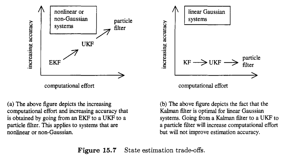
• Particle filter is the complete nonlinear filter unlike EKF or UKF. This can be used when the system’s nonliearity is severe.

• The drawback of this filter is its computational bottleneck. Below figure describes it.

State estimation trade-off

Simon, Dan. 2006. Optimal State Estimation: Kalman, h Infinity, and Nonlinear Approaches. John Wiley & Sons.