1 Abstract
This work presents detailed steps on solving one-dimensional heat conduction equation incorporating both Dirichlet and Neumann type boundary conditions using the Theory of Functional Connections. The polynomial series was used as the free function in the constrained expression. The resulting matrix equation was solved using both pseudo-inverse and QR decomposition methods. Further, the error analysis was performed on both the methods by varying the number of colocation points and number of terms in the polynomial series. The solution obtained using QR decomposition was found to be well accurate, having an L_2 error norm of order 10^{-12}. While, the pseudo-inverse was yielding less accurate results due to high condition number on the coefficient matrix.
2 Introduction
The Theory of Functional Connections (TFC) is a mathematical framework for functional interpolation invented by Mortari (2017). It is a procedure to derive a parametric expression, called as constrained expression that approximates the given scalar function, similar to other functional interpolation methods like fourier series.
However, the constrained expressions are unique among functional interpolation methods due to their intrinsic embedding of the linear constraints imposed on the scalar function. Thus, the constraints are always satisfied to machine precision, independent of the parameters in the constrained expression. The general form of constrained expression is given as
y(x) = g(x) + \sum_{i=1}^{N_c} \phi_i(x) \rho_i\left(x,g(x)\right) \ . \tag{1}
Here, y(x) is the given function that has to be modeled. The g(x) is called as the free function. This function will have the parameters to be estimated to approximate y(x) accurately. Some examples of g(x) are fourier series, Chebyshev polynomials and neural networks. \phi(x) is called as the switching function which is a continuous function that returns 1 at the corresponding constraint location and returns 0 at other constraint locations in the domain. \rho(x,g(x)) is called as the projection functional, that projects the free function g(x) on to the set of functions that vanish at the constraint location in the domain. More details on these constrained expressions can be found in Johnston (2021).
One of the popular approaches to solve a differential equation is the spectral methods, where the solution is assumed to be a combination of finite number of continuous functions. Solving a differential equation requires initial and boundary conditions to be specified, which is mostly dirichlet and neumann type conditions. So, the assumed solution function should also satisfy these conditions along with the differential equation.
The main advantage of spectral methods over numerical integration is that the spectral methods give a continuous function as solution, overcoming the domain discretization related issues. But, solving the differential equation using spectral methods is a regression process. The parameters present in the assumed solution function are the design variables with the residual form of the differential equation as the objective function. The solution function to the differential equation is obtaind by minimizing the objective function by optimizing the function parameters.
When viewing regression as a solution method to the equations, a fundamental problem with the regression can be observed. A function obtained through regression will not pass through all the data points, including the points induced by the boundary conditions (dirichlet type conditions for example). Whereas, interpolation process will make the function to pass through all the points, including noise data points.
A hybrid approach that combines the advantages of interpolation (constraint satisfaction) and regression (best fitting of function) would leverage the spectral solution methods to the differential equations. Fortunately, the Theory of Functional Connections is seen as the aforementioned hybrid approach. The modelled function satisfies the boundary conditions (seen as constraints) to machine precision while still flexible to fit to the actual solution function.
As mentioned before, an deep explanation withe examples on deriving constrained expressions for various constraint types can be seen in Johnston (2021), and the application of TFC to solve differential equations can be seen in Mortari, Johnston, and Smith (2019). In this work, an indepth explanation of solving a 2nd order differential equation using TFC is provided, covering key points on the derivation of constrained expression and error analysis on the solution which were not covered in the literature.
3 Problem definition
In this work, the 1D heat conduction equation with source subjected to the fixed temperature value (Dirichlet condition) on one side and the fixed temperature gradient (Neumann condition) on the other side is solved using the Theory of functional connections. The equation is
k \frac{d^2 T}{dx^2} + q = 0, \ \ x\in[0,1], \tag{2}
with the boundary conditions T(0) = 0 and dT/dx|_{x=1} = 2\cos(2). Motive of the present work is to demonstrate the TFC application to present problem and to analyze the accuracy on the solution of the method. The traditional approach to perform error analysis is to compare the computed solution with some benchmark problem solution. However, an elegant approach will be to use the method of manufactured solutions (MMS) (Roache (2002)). So, the MMS will be used for validating the computation code and solution methodology.
3.1 Method of Manufactured Solutions (MMS)
A general outline of the MMS is as follows: first, an analytical function for the dependent variable is framed that would be consistent with the calculus operations involved in the equation. Then, the analytical function is substituted in the equation, performing all the calculus operations leading to an algbraic expression equating to zeros. Finally, the resulting expression with opposite sign is taken as the source term of the equation, thus the function is satisfying the equation exactly. The manufactured solution need not be scientifically feasible but should satisfy the equations.
For the Equation 2, the simplest manufactured solution taken is T_m(x) = \sin(2x)\ \ \ x \in[0,1] \ . \tag{3}
Substituting Equation 3 in Equation 2 yields the expression for the source term q as shown below.
\begin{align*} k \frac{d^2}{dx^2}\left(\sin(2x)\right) + q &= 0 \\ - k \times 4 \times \sin(2x) + q &= 0 \\ -4k\sin(2x) + q &= 0 \\ q &= 4k\sin(2x) \end{align*}
Taking k=1 and substituting the above derived source term expression into Equation 2 gives
\frac{d^2 T}{dx^2} + 4\sin(2x) = 0 \ . \tag{4}
Thus the exact solution to Equation 4 is Equation 3. It can also be seen that the manufactured solution satisfies the constraint i.e. boundary conditions specified. T_m(0) = 0 and dT_m/dx|_{x=1}=2\cos(2). In fact, the manufactured solution was first prepared for this work and the boundary conditions were back-calculated from that, with the motive of having one Dirichlet and one Neumann boundary conditions.
Now that the problem to be solved is defined and the expected solution with appropriate boundary conditions were manufactured, the next step is to derive the constrained expression T_{ce} by using the Theory of Functional Connections.
4 Constrained Expression derivation
The general form of the constrained expression is given in Equation 1. The present problem has two constraints, so re-writing the general expression into problem-specific as
T_{ce}(x) = g(x) + \phi_1(x)\rho_1(x,g(x)) + \phi_2(x)\rho_2(x,g(x)) \ . \tag{5}
Here, \phi_1(x) and \rho_1(x,g(x)) are the switching function and projection functional respectively for the Dirichlet condition T(0)=0. \phi_2(x) and \rho_2(x,g(x)) are the switching function and projection functional respectively for the Neumann condition dT/dx|_{x=1}=2\cos(2).
Now, following the dissertation of Johnston (2021), the switching functions \phi_1(x), \phi_2(x) are made as linear combination of support functions s_1(x),s_2(x). Support functions can be of any mathematical function that has to satisfy one property: support functions have to be defined on all the constraint locations.
When TFC is applied for solving the differential equation, the support functions have to be chosen such that they are atleast differentiable to the highest order seen in the differential equation.
This ensures that the constraint terms appear in the final algebraic expression obtained after substituting the constrained expression in the differntial equation.
There should be as many support functions as the switching functions or number of constraints. Following the above personal observation, the Equation 4 is a second order differential equation. Hence, the support functions have to be atleast twice differentiable without going to zero.
Now, we know that the switching functions are the continuous functions that will return one at appropriate constraint location and will return zero at other constriant locations. And the switching functions are linear combinations of support functions.
So, taking \phi_1(x) and at x=0, \phi_1(0) = 1. The condition is T(0)=0 which is a Dirichlet type condition. Hence, \phi_1(x) at x=0 can be written as
\phi_1(0) = \alpha_{1,1} s_1(0) + \alpha_{2,1} s_2(0) = 1 \ . \tag{6}
Similarly, taking \phi_1(x) and at x=1, d\phi_1/dx|_{x=1} = 0. Note that the derivative of \phi_1(x) at x=1 is zero and \phi_1(1) \ne 0, because the condition given is Neumann type, dT/dx|_{x=1}=2\cos(2). Hence, \phi_1(x) at x=1 can be written as,
\begin{align*} \frac{d \phi_1}{dx}\Bigg\lvert_{x=1} &= \alpha_{1,1} \frac{d s_1}{dx}\Bigg\lvert_{x=1} + \alpha_{2,1} \frac{d s_2}{dx}\Bigg\lvert_{x=1} = 0\\ &= \alpha_{1,1} s_{1,x}(1) + \alpha_{2,1} s_{2,x}(1) = 0\\ \end{align*} \tag{7}
The Equation 6 and Equation 7 can be writen as a single matrix equation as
\begin{bmatrix} \phi_1(0) \\ \frac{d \phi_1}{dx}\lvert_{x=1} \end{bmatrix} = \begin{bmatrix} s_1(0) & s_2(0) \\ s_{1,x}(1) & s_{2,x}(1) \end{bmatrix} \begin{bmatrix} \alpha_{1,1} \\ \alpha_{2,1} \end{bmatrix} = \begin{bmatrix} 1 \\ 0 \end{bmatrix} \ . \tag{8}
Now, taking \phi_2(x) and at x=0, \phi_2(0)=0. So, writing phi_2(x) as
\phi_2(0) = \alpha_{1,2} s_1(0) + \alpha_{2,2} s_2(0) = 0 \ . \tag{9}
Similarly, taking \phi_2(x) at x=1, d\phi_2/dx|_{x=1}=1. So, writing \phi_2(x) at x=1 as
\frac{d \phi_2}{dx}\Bigg\lvert_{x=1} = \alpha_{1,2} s_{1,x}(1) + \alpha_{2,2} s_{2,x}(1) = 1 \ . \tag{10}
Combining Equation 9 and Equation 10 into matrix form as
\begin{bmatrix} \phi_2(0) \\ \frac{d \phi_2}{dx}\lvert_{x=1} \end{bmatrix} = \begin{bmatrix} s_1(0) & s_2(0) \\ s_{1,x}(1) & s_{2,x}(1) \end{bmatrix} \begin{bmatrix} \alpha_{1,2} \\ \alpha_{2,2} \end{bmatrix} = \begin{bmatrix} 0 \\ 1 \end{bmatrix} \ . \tag{11}
Further, the Equation 8 and Equation 11 can be combined together as
\begin{bmatrix} \phi_1(0) & \phi_2(0) \\ \frac{d \phi_1}{dx}\lvert_{x=1} & \frac{d \phi_2}{dx}\lvert_{x=1} \end{bmatrix} = \begin{bmatrix} s_1(0) & s_2(0) \\ s_{1,x}(1) & s_{2,x}(1) \end{bmatrix} \begin{bmatrix} \alpha_{1,1} & \alpha_{1,2} \\ \alpha_{2,1} & \alpha_{2,2} \end{bmatrix} = \begin{bmatrix} 1 & 0 \\ 0 & 1 \end{bmatrix} \ . \tag{12}
Here, the \alpha_{1,1},\alpha_{1,2},\alpha{2,1} and \alpha_{2,2} are the unknown scalars to be computed. In order to compute the unknown \alpha’s, the column vectors of support function matrix: [s_1(0) \ s_{1,x}(1)]^T and [s_2(0) \ s_{2,x}(1)]^T should be linearly independent, so that the unknowns can be computed by taking inverse of support function matrix.
In this work, the support functions are chosen as s_1(x) = e^x and s_2(x) = e^{2x}, because they are linearly independent, easy to differentiate, infinitely differentiable and yield small manageable values within the domain x\in[0,1].
Substituting the support functions in Equation 12 and evaluated at the constraint locations gives
\begin{bmatrix} \phi_1(0) & \phi_2(0) \\ \frac{d \phi_1}{dx}\lvert_{x=1} & \frac{d \phi_2}{dx}\lvert_{x=1} \end{bmatrix} = \begin{bmatrix} 1 & 1 \\ e & 2e \end{bmatrix} \begin{bmatrix} \alpha_{1,1} & \alpha_{1,2} \\ \alpha_{2,1} & \alpha_{2,2} \end{bmatrix} = \begin{bmatrix} 1 & 0 \\ 0 & 1 \end{bmatrix} \ . \tag{13}
Solving above equation for \alpha’s give \begin{align*} \alpha_{1,1} &= \frac{2e}{2e-1} \\ \alpha_{1,2} &= \frac{-1}{2e^2-e} \\ \alpha_{2,1} &= \frac{-1}{2e-1} \\ \alpha_{2,2} &= \frac{1}{2e^2-e} \end{align*} \tag{14}
Hence, the complete switching functions expressions are \begin{align*} \phi_1(x) &= \left(\frac{2e}{2e-1}\right)e^x + \left(\frac{-1}{2e-1}\right)e^{2x} \\ \phi_2(x) &= \left(\frac{-1}{2e^2-e}\right)e^x + \left(\frac{1}{2e^2-e}\right)e^{2x} \end{align*} \tag{15}
Now, again following Johnston (2021), the projection functionals for the present problem will be
\begin{align*} \rho_1(x,g(x)) &= T(0) - g(0) \\ \rho_2(x,g(x)) &= \frac{d T}{dx}\Bigg\lvert_{x=1} - g_x(1) \end{align*} \tag{16}
So, substituting Equation 15 and Equation 16 into Equation 5 yeilds the semi-complete form of constrained expression as
\begin{equation} \begin{split} T_{ce}(x) = g(x) + \left(\left(\frac{2e}{2e-1}\right)e^x + \left(\frac{-1}{2e-1}\right)e^{2x} \right)\left(T(0) - g(0)\right) + \\ \left(\left(\frac{-1}{2e^2-e}\right)e^x + \left(\frac{1}{2e^2-e}\right)e^{2x}\right)\left(\frac{dT}{dx}\Bigg\lvert_{x=1}-g_x(1)\right) \end{split} \end{equation} \tag{17}
It is semi-complete because, the free function g(x) is not yet defined. The general N_kth degree polynomial expression is chosen as the free function. It is given as g(x) = \sum_{k=0}^{N_k}a_k x^k , \ x\in[0,1] \ . \tag{18}
It can be noted that, there exists first order derivative of free function g_x(1) evaluated at x=1 in the Equation 17. Computing the first derivative of Equation 18 as g_x(x) = \sum_{k=0}^{N_k}a_k k x^{k-1} , \ x \in[0,1] \ . \tag{19}
When programming Equation 19, the zeroDivisionError will occur for k=0 at x=0. However, the value of g_x(0) is zero as the multiple, k=0. So, appropriate steps need to be taken in the code, for example, by adding a very small value \epsilon to the x for k=0 case.
Thus, the complete constrained expression is obtained by substituting Equation 18, and Equation 19 evaluated at x=0 \ \& \ x=1, into Equation 17 as
\begin{equation} \begin{split} T_{ce}(x) = \sum_{k=1}^{N_k}a_kx^k + \left(\left(\frac{2e}{2e-1}\right)e^x + \left(\frac{-1}{2e-1}\right)e^{2x} \right)\left(T(0) - \sum_{k=1}^{N_k}a_k[0]^k\right) + \\ \left(\left(\frac{-1}{2e^2-e}\right)e^x + \left(\frac{1}{2e^2-e}\right)e^{2x}\right)\left(\frac{dT}{dx}\Bigg\lvert_{x=1}-\sum_{k=1}^{N_k}a_k k [1]^{k-1}\right) \end{split} \end{equation} \tag{20}
The unknowns in the above equation are a_k’s. However, the constraint is always satisfied independent of a_k values. So, the a_k values can be optimized to satisfy the governing equation alone. Thus, the constrained optimization problem is converted to an unconstrained one with TFC.
Now that the constrained expression is obtained, the next step is to frame the algebraic expression and solve for the unknown a_k’s.
5 Solving the problem using TFC
In order to solve the Equation 4, the constrained expression just derived (Equation 20) has to be substituted on to Equation 4 and the resulting algebraic expression has to be solved for the unknown parameters \alpha’s.
It can be noted that the Equation 4 has a 2nd order derivative of the dependent function T. For simplistic derivation, lets take Equation 17 and differentiate w.r.t. x, that gives
\begin{equation*} \begin{split} \frac{d T_{ce}}{dx} = g_x(x) + \left(\frac{2e}{2e-1}e^x +\frac{-2}{2e-1}e^{2x}\right) \left(T(0) - g(0)\right) + \\ \left(\frac{4e^{2x}}{2e^2-e}-\frac{e^x}{2e^2-e}\right) \left(\frac{dT}{dx}\Bigg\lvert_{x=1} - g_x(1)\right) \end{split} \end{equation*}
Taking second derivative of above equation gives
\begin{equation} \begin{split} \frac{d^2T_{ce}}{dx^2} = g_{xx}(x) + \left(\frac{2e}{2e-1}e^x-\frac{4}{2e-1}e^{2x}\right) \left(T(0)-g(0)\right) + \\ \left(\frac{4e^{2x}}{2e^2-e}-\frac{e^x}{2e^2-e}\right) \left(\frac{dT}{dx}\Bigg\lvert_{x=1} - g_x(1)\right) \end{split} \end{equation} \tag{21}
Now, handling the free function separately as \begin{align*} g(x) &= \sum_{k=0}^{N_k} a_k x^k \\ g_x(x) &= \sum_{k=0}^{N_k} a_k k x^{k-1} \\ g_{xx}(x) &= \sum_{k=0}^{N_k} a_k (k^2-k) x^{k-2} \end{align*} \tag{22}
Now, substituting above equation in Equation 21 and then substituting resulting expression into Equation 4 gives
\begin{equation} \begin{split} \sum_{k=0}^{N_k} a_k (k^2-k) x^{k-2} + \left(\frac{2e}{2e-1}e^x-\frac{4}{2e-1}e^{2x}\right) \left(T(0) - \sum_{k=0}^{N_k}a_k [0]^k\right) + \\ \left(\frac{4e^{2x}}{2e^2-e}-\frac{e^x}{2e^2-e}\right) \left(\frac{dT}{dx}\Bigg\lvert_{x=1} - \sum_{k=0}^{N_k}a_k k [1]^{k-1}\right) + 4\sin(2x) = 0 \end{split} \end{equation} \tag{23}
For shortening the expression, let \begin{align*} \phi_1''(x) &= \left(\frac{2e}{2e-1}e^x - \frac{4}{2e-1}e^{2x}\right) \\ \phi_2''(x) &= \left(\frac{4e^{2x}}{2e^2-e} - \frac{e^x}{2e^2-e}\right) \ . \end{align*}
Then the Equation 23 becomes
\begin{equation*} \begin{split} \sum_{k=0}^{N_k} a_k (k^2-k) x^{k-2} + \phi_1''(x) \left(T(0) - \sum_{k=0}^{N_k}a_k [0]^k\right) + \\ \phi_2''(x) \left(\frac{dT}{dx}\Bigg\lvert_{x=1} - \sum_{k=0}^{N_k}a_k k [1]^{k-1}\right) + 4\sin(2x) = 0 \ . \end{split} \end{equation*}
Combining the terms having a_k into one term in the above equation,
\begin{equation*} \begin{split} \sum_{k=0}^{N_k}a_k\left[(k^2-k)x^{k-2}-\phi_1''(x)[0]^k-\phi_2''(x)k [1]^{k-1}\right] + \\ \phi_1''(x) T(0) + \phi_2''(x)\frac{dT}{dx}\Bigg\lvert_{x=1} + 4\sin(2x) = 0 \ . \end{split} \end{equation*}
Replacing sumation with vector product and taking scalar term on the other side as, \begin{equation} \begin{split} \mathbf{a}^T\left[(k^2-k)x^{k-2}-\phi_1''(x)[0]^k-\phi_2''(x)k [1]^{k-1}\right]_{k=0}^{N_k} \\ = - \phi_1''(x) T(0) - \phi_2''(x)\frac{dT}{dx}\Bigg\lvert_{x=1} - 4\sin(2x) \ . \end{split} \end{equation} \tag{24}
For further simplification, let \begin{align*} \mathbf{h}(x) &= \left[(k^2-k)x^{k-2}-\phi_1''(x)[0]^k-\phi_2''(x)k [1]^{k-1}\right]_{k=0}^{N_k} \\ y(x) &= - \phi_1''(x) T(0) - \phi_2''(x)\frac{dT}{dx}\Bigg\lvert_{x=1} - 4\sin(2x) \ . \end{align*}
Note that, \mathbf{h}(x) is a vector function and y(x) is a scalar function. Then, substituting the above equations in Equation 24 gives
\mathbf{a}^T \mathbf{h}(x) = y(x) \tag{25}
Now, let the domain x\in[0,1] be discretized into N colocation points: {x_1,x_2,\dots,x_N}. And, let \mathbf{h}_1 = \mathbf{h}(x_1), \mathbf{h}_2 = \mathbf{h}(x_2), \dots \mathbf{h}_N = \mathbf{h}(x_N) and y_1 = y(x_1), y_2 = y(x_2), \dots y_N = y(x_N). Substituting the Equation 25 from functional form to algebraic form by augmenting the \mathbf{h}’s and y’s for all colocation points as
\begin{equation*} \mathbf{a}^T\left[\mathbf{h}_1 \ \mathbf{h}_2 \ \dots \ \mathbf{h}_N\right] = \left[y_1 \ y_2 \ \dots \ y_N\right] \end{equation*}
Performing further manipulations on the above equation, \begin{align*} \left[\mathbf{a}^T\left[\mathbf{h}_1 \ \mathbf{h}_2 \ \dots \ \mathbf{h}_N\right] \right]^T &= \left[y_1 \ y_2 \ \dots \ y_N\right]^T \\ \left[\mathbf{h}_1 \ \mathbf{h}_2 \ \dots \ \mathbf{h}_N \right]^T\mathbf{a} &= \left[y_1 \ y_2 \ \dots \ y_N\right]^T \\ \mathbf{H} \mathbf{a} &= \mathbf{y} \end{align*}
Hence the expression \boxed{\mathbf{H}\mathbf{a} = \mathbf{y}} \tag{26}
is the final algebraic expression, where \mathbf{H} is called as the coefficient matrix, \mathbf{y} is the source vector and \mathbf{a} is the unknown vector. It is of the form \mathbf{A}\mathbf{x}=\mathbf{b}, which is a standard equation in mathematics that has multiple solution methods. In this work, two of the solution methods were compared: pseudo-inverse of \mathbf{H}, and QR decomposition.
5.1 Solution to the problem
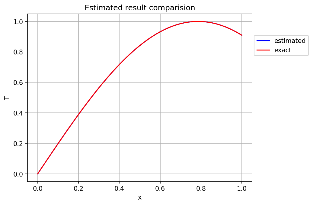
The Equation 26 was solved with the number of terms in polynomial N_k = 51 and the number of colocation points N=51. First the method of using pseudo-inverse was applied and the Figure 1 shows the visual comparison of estimated and expected results.

The results match perfectly visually, thus the absolute difference between both the profiles was computed and ploted, shown in Figure 2.
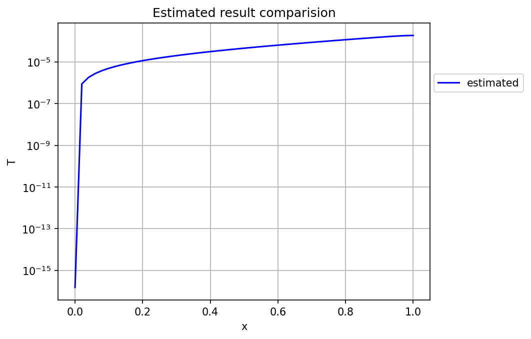
It can be seen in the above graph that the max error is in the range of 10^{-5}. Moreover, the L_2 error of the result is 8.45\times10^{-5}. The error obtained is relatively high for the simple problem and the reason for this is the high condition number of the coefficient matrix \mathbf{H}, which is about 7\times10^{18}.
The QR decomposition method is preferred for the system with high condition number as the coefficient matrix \mathbf{H} is split into two matrices: an orthonormal matrix \mathbf{Q}, an upper triangular matrix \mathbf{R}. Thus, the Equation 26 can be writen as
\mathbf{H}\mathbf{a} = \mathbf{Q}\mathbf{R}\mathbf{a} = \mathbf{y}
Computing inverse of \mathbf{Q} is accurate as its condition number will be \approx 1 resulting in the equation \begin{align*} \mathbf{Q}\mathbf{R}\mathbf{a} &= \mathbf{y} \\ \mathbf{R}\mathbf{a} &= \mathbf{Q}^{-1}\mathbf{y} \\ \mathbf{R}\mathbf{a} &= \tilde{\mathbf{y}} \\ \end{align*}
Since \mathbf{R} is an upper triangular matrix, the last above equation can be solved for \mathbf{a} by back-substitution method. The visual comparison of result obtained using QR decomposition method with the manufactured solution is given below.
Again, the visual comparison shows matching results. Hence, the absolute error plot was made and shown in Figure 4.
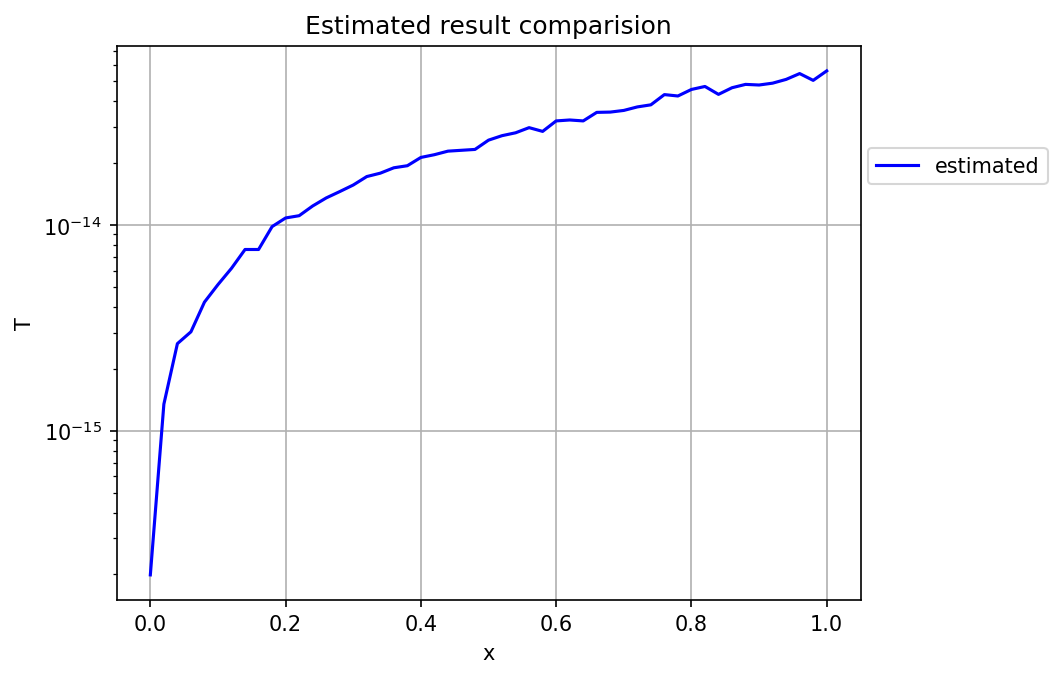
It was observed that the QR decomposition method gave much accurate results both from the above graph and from its L_2 error norm which is \approx 3\times10^{-14}.
The Python code used in this problem computation can be found here.
#!/bin/python3
"""============================================================================
Solution of 1D HC equation with dirichlet and neumann bcs using TFC

Ramkumar
Wed Jun 18 10:47:55 AM IST 2025
============================================================================"""

# importing needed modules
import numpy as np
import pandas as pd
import matplotlib.pyplot as plt
from numpy import e as e

#==============================================================================

##
N       = 51              # number of data points
Nk      = 51              # number of terms in sine series
L       = 1.0             # domain length
x0      = 0               # location of left bc
xL      = L               # location of right bc
Tx0     = 0               # value of T at left bc
dTdx_xL = 2*np.cos(2*xL)  # value of dTdx at right bc

# manufactured solution
Tm = lambda x: np.sin(2*x)

# source term in heat equation
q = lambda x: 4*np.sin(2*x)

# defining domain colocation points
x = np.linspace(x0+1e-15,xL,N)  # +1e-15 to prevent zeroDivisionError

# defining switching functions
phi1 = lambda x: (2*e/(2*e-1))*e**x + (-1/(2*e-1))*e**(2*x)
phi2 = lambda x: e**(2*x)/(2*e**2-e) - e**x/(2*e**2-e)

phi1_dd = lambda x: 2*e*e**x/(2*e-1) - 4/(2*e-1)*e**(2*x)
phi2_dd = lambda x: 4*e**(2*x)/(2*e**2-e) - e**x/(2*e**2-e)

# computing y vector
y = np.zeros(N)
for i in range(N):
    y[i] = -4*np.sin(2*x[i])-phi1_dd(x[i])*Tx0-phi2_dd(x[i])*dTdx_xL

# computing H matrix
H = np.zeros([N,Nk])
for i in range(N):
    for k in range(Nk):
        H[i,k] = ( (k**2-k)*x[i]**(k-2) -
                    phi1_dd(x[i])*x0**k -
                    phi2_dd(x[i])*k*xL**(k-1) )

H = np.nan_to_num(H,0)

# printing condition number of H
print("Condition number of H = ",np.linalg.cond(H))

# # computing coefficients using pseudo-inverse
# a = np.linalg.pinv(H)@y

# computing coefficients using QR decomposition
a = np.zeros(Nk)
Q,R = np.linalg.qr(H)
y_tilda = np.linalg.pinv(Q)@y
a[Nk-1] = y_tilda[Nk-1]/R[Nk-1,Nk-1]
for i in reversed(range(Nk-1)):  # back substitution
    sumVal = 0
    for k in reversed(range(i+1,Nk)):
        sumVal += R[i,k]*a[k]
    a[i] = (y_tilda[i]-sumVal)/R[i,i]


# computing CE solution vector
T_CE = np.zeros(N)
for i in range(N):
    T_CE[i] += np.sum([a[k]*x[i]**k for k in range(Nk)])
    T_CE[i] += phi1(x[i])*(Tx0 - np.sum([a[k]*x0**k for k in range(Nk)]))
    T_CE[i] += phi2(x[i])*(dTdx_xL-np.sum([a[k]*k*xL**(k-1) for k in range(Nk)]))

# plotting graphs for comparison

plt.figure()
plt.plot(x,T_CE,'-b',label="estimated")
plt.plot(x,Tm(x),'-r',label="exact")
plt.grid()
plt.xlabel("x")
plt.ylabel("T")
plt.title("Estimated result comparision")
plt.legend(loc=(1.01,0.75))
plt.savefig("output.png",dpi=150,bbox_inches="tight")

plt.figure()
plt.plot(x,np.abs(T_CE-Tm(x)),'-b',label="estimated")
plt.grid()
plt.xlabel("x")
plt.ylabel("T")
plt.title("Estimated result comparision")
plt.legend(loc=(1.01,0.75))
plt.yscale("log")
plt.savefig("errorPlot.png",dpi=150,bbox_inches="tight")
plt.show()

print("\n L2 error = ",np.sqrt(np.mean(np.square(T_CE-Tm(x)))))

#==============================================================================
However, this computation is done for the number of colocation points N=51 and the number of terms in polynomial N_k=51. In order to assert the performance of the solver model, the L_2 errors of both methods (pseudo-inverse and QR) and the condition number of \mathbf{H} matrix have to be evaluated for a range of N and N_k combinations, which is done in the next section.
6 Error analysis
To assert the performance of the solver model developed, the L_2 errors of both solution methods and the condition number of \mathbf{H} matrix were computed for the range N\in[5,6,7,\dots,101] and N_k\in[5,6,7,\dots,101]. However, there is this restriction: N_k \le N, otherwise the equation system will be under-determined.
Hence, the series of computations were performed for the possible combinations of N and N_k, and the resulting errors and condition numbers were plotted as contours that are given below.
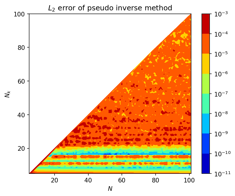
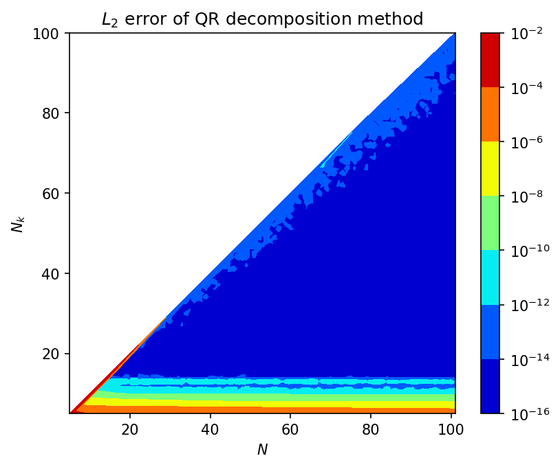
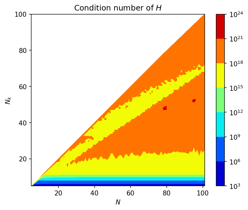
It can be seen from Figure 5 that the overall maximum error of the pseudo-inverse method is in the order of 10^{-5} to 10^{-3}. And a few regions of error in the order of 10^{-11} were observed. The corresponding regions in the Figure 7 show high condition number for the (N,N_k) combinations. This is in correspondence with the theory that the pseudo inverse of a high conditioned matrix will be less accurate.
The overall maximum error of the QR decomposition method is close to machine precision 10^{-16} to 10^{-14} despite the high condition number. See Figure 6. This is due to spliting of \mathbf{H} into an ortho-normal matrix \mathbf{Q} and an upper triangular matrix \mathbf{R}. Inverting \mathbf{Q} will be accurate and an easy back-substitution method can be used to solve for unknown vector \mathbf{a} with the \mathbf{R} matrix. Hence, QR decomposition method is useful.
Further, one observation from the QR decomposition error contour (Figure 6) is that the accurate results were obtained in the region N_k\approx N/2. This could be problem specific, but was observed for other problems tried. So, for now, selecting N_k to be the half of N with N being sufficiently large (N>10 for this problem) can yield accurate results.
The other thing observed from condition number contour (Figure 7) that the relatively low condition number paired with low error on QR decomposition method was following two patterns: one is N\approx 20 for the range of N, and the other is N_k\le\frac{3}{4}N.
The Python code developed for this error analysis can be seen here
#!/bin/python3
"""============================================================================
Solution of 1D HC equation with dirichlet and neumann bcs using TFC

Ramkumar
Wed Jun 18 10:47:55 AM IST 2025
============================================================================"""

# importing needed modules
import numpy as np
import pandas as pd
import matplotlib.pyplot as plt
from numpy import e as e

#==============================================================================

# solver function definition
def solverFunction(N,Nk):
    L       = 1.0             # domain length
    x0      = 0               # location of left bc
    xL      = L               # location of right bc
    Tx0     = 0               # value of T at left bc
    dTdx_xL = 2*np.cos(2*xL)  # value of dTdx at right bc

    # manufactured solution
    Tm = lambda x: np.sin(2*x)

    # source term in heat equation
    q = lambda x: 4*np.sin(2*x)

    # defining domain colocation points
    x = np.linspace(x0+1e-15,xL,N)  # +1e-15 to prevent zeroDivisionError

    # defining switching functions
    phi1 = lambda x: (2*e/(2*e-1))*e**x + (-1/(2*e-1))*e**(2*x)
    phi2 = lambda x: e**(2*x)/(2*e**2-e) - e**x/(2*e**2-e)

    phi1_dd = lambda x: 2*e*e**x/(2*e-1) - 4/(2*e-1)*e**(2*x)
    phi2_dd = lambda x: 4*e**(2*x)/(2*e**2-e) - e**x/(2*e**2-e)

    # computing y vector
    y = np.zeros(N)
    for i in range(N):
        y[i] = -4*np.sin(2*x[i])-phi1_dd(x[i])*Tx0-phi2_dd(x[i])*dTdx_xL

    # computing H matrix
    H = np.zeros([N,Nk])
    for i in range(N):
        for k in range(Nk):
            H[i,k] = ( (k**2-k)*x[i]**(k-2) -
                        phi1_dd(x[i])*x0**k -
                        phi2_dd(x[i])*k*xL**(k-1) )

    H = np.nan_to_num(H,0)

    # computing coefficients using pseudo-inverse
    a_pinv = np.linalg.pinv(H)@y

    # computing coefficients using QR decomposition
    a_qr = np.zeros(Nk)
    Q,R = np.linalg.qr(H)
    y_tilda = np.linalg.pinv(Q)@y
    a_qr[Nk-1] = y_tilda[Nk-1]/R[Nk-1,Nk-1]
    for i in reversed(range(Nk-1)):  # back substitution
        sumVal = 0
        for k in reversed(range(i+1,Nk)):
            sumVal += R[i,k]*a_qr[k]
        a_qr[i] = (y_tilda[i]-sumVal)/R[i,i]


    # computing CE solution vector
    T_CE_pinv = np.zeros(N)
    T_CE_qr = np.zeros(N)
    for i in range(N):
        T_CE_pinv[i] += np.sum([a_pinv[k]*x[i]**k for k in range(Nk)])
        T_CE_pinv[i] += phi1(x[i])*(Tx0 - np.sum([a_pinv[k]*x0**k for k in range(Nk)]))
        T_CE_pinv[i] += phi2(x[i])*(dTdx_xL-np.sum([a_pinv[k]*k*xL**(k-1) for k in range(Nk)]))

        T_CE_qr[i] += np.sum([a_qr[k]*x[i]**k for k in range(Nk)])
        T_CE_qr[i] += phi1(x[i])*(Tx0 - np.sum([a_qr[k]*x0**k for k in range(Nk)]))
        T_CE_qr[i] += phi2(x[i])*(dTdx_xL-np.sum([a_qr[k]*k*xL**(k-1) for k in range(Nk)]))

    L2_pinv = np.sqrt(np.mean(np.square(T_CE_pinv-Tm(x))))
    L2_qr   = np.sqrt(np.mean(np.square(T_CE_qr-Tm(x))))
    cNo     = np.linalg.cond(H)

    print(N,"\t",Nk)

    return L2_pinv,L2_qr,cNo

## computing data

fid = open("errorData.csv","w")  # creating data file and writing header
fid.writelines("N,Nk,L2_pinv,L2_qr,cNo\n")
fid.close()

# creating design space grid
Ngrid = 101
Ng,Nkg = np.meshgrid(np.linspace(5,101,Ngrid,dtype=int),
                   np.linspace(5,101,Ngrid,dtype=int))
N_list = []
Nk_list = []
for i in range(Ngrid):
    for j in range(i):
        N_list.append(Ng[j,i])
        Nk_list.append(Nkg[j,i])

# performing computation
for (N,Nk) in zip(N_list,Nk_list):
    L2_pinv,L2_qr,cNo = solverFunction(N,Nk)
    fid = open("errorData.csv","a")
    data = str(N)+","+str(Nk)+","+str(L2_pinv)+","+str(L2_qr)+","+str(cNo)+"\n"
    fid.writelines(data)
    fid.close()


#==============================================================================
7 Conclusion
The aim of demonstrating the application of the Theory of Functional Connections (TFC) to solve differential equations involving both Dirichlet and Neumann type boundary conditions was accomplished through this work. The 1D heat conduction equation was chosen for the work with fixed temperature on one side and the temperature gradient on the other side. The method of manufactured solutions was used to create a manufactured solution that satisfies the heat conduction equation exactly, so that the error analysis on the TFC method can be performed.
An in-depth explanation on advantages of the constrained expressions and its derivation using general polynomial expression as free function for the present problem was provided. Further, the derived constrained expression was substituted in the governing equation and obtained the final algebraic expression. The obtained algebraic expression was then solved with two methods: pseudo-inverse and QR decomposition. The performance comparison was performed on both the methods for a range of number of colocation points and the number of terms in the polynomial series. The QR decomposition method was found to perform better due to high condition number of the coefficient matrix in the algebraic expression.
This work was made to be used as a base reference for further computations involving TFC to solve differential equations. Python codes developed for this work were embedded inline this manuscript, given as open to the reader. Futher, the research on applying TFC to solve multi-variate and vector functions is kept as the direction of future work.