Introduction to Neural Networks

Multi-Disciplinary Optimization Course

2025-04-22

Content

Section 1: Neuron, Neural network and forward propagation

Section 2: Weights initialization, loss functions and back-propagation

Section 3: Data normalization and Optimization algorithms

1 Neuron, neural networks and forward propagation

1.1 Neuron

A linear/non-linear function that takes in multiple inputs and produces one output.

\[ y = f\left( w_1\times x_1 + w_2\times x_2 + \dots + w_n \times x_n + w_0\right) \]

\[ y = f\left(\sum_{i=1}^n w_i x_i + w_0 \right) = f\left(\textbf{w}^T\textbf{x} + w_0\right) \]

1.2 Activation functions

The purpose of activation function is to induce non-linearity into the model.

Let \(z = \textbf{w}^T\textbf{x}+w_0\),

\(z\) is called pre-activation vector (or scalar), \(\textbf{w} = \{w_1,\dots,w_n\}\) and \(\textbf{x} = \{x_1,\dots,x_n\}\)

\[ y = f\left(z\right) \]

It has a linear component \(z\) covered by a non-linear function \(f\)
Some of the activation functions
- Rectified Linear Unit (ReLU), \(y = max(0,z)\)
- Sigmoid function, \(y = \frac{1}{1+exp(-z)}\)
- Hyperbolic tan function, \(y = tanh(z)\)

1.3 Neural Network

Engineering problems will require functions with multiple outputs for a set of inputs
Example: 2D incompressible flow over flat plate. \(f_{NN}: x,y \to u,v,p\)

for each blue neuron in hidden layer in the schematic, \(z_j = \textbf{w}^T_j\textbf{x} + w_{0,j},\;\; j=1,2,3,4; \; \; \textbf{x}=\{x,y\}^T\)
In matrix form, it will be \[ \begin{bmatrix}z_1 \\ z_2 \\ z_3 \\ z_4\end{bmatrix} = \begin{bmatrix} \textbf{w}_1^T \\ \textbf{w}_2^T \\ \textbf{w}_3^T \\ \textbf{w}_4^T \end{bmatrix} \begin{bmatrix} x \\ y \end{bmatrix} + \begin{bmatrix} w_{0,1} \\ w_{0,2} \\ w_{0,3} \\ w_{0,4} \end{bmatrix} \] \[ \textbf{z} = \textbf{W}\textbf{x}+\textbf{b} \]

\(\textbf{z},\textbf{b}\) are \((4\times 1)\) vector, \(\textbf{x}=\{x,y\}^T\) is \((2\times 1)\) input vector and \(\textbf{W}\) is \((4\times 2)\) weight matrix

1.4 Universal Approximation Theorem (Cybenkov 1989)

Theorem 1 Let \(I_n\) denote the n-dimensional unit cube \([0,1]^T\) and \(C(I_n)\) be the space of continuous functions defined in \(I_n\). Let \(x\in\mathbb{R}^n\) and \(\sigma\) be any continuous discriminatory function. Then the finite sums of the form

\[ G(x) = \sum_{j=1}^N \alpha_j \sigma(y_j^T x + \theta_j) \]

are dense in \(C(I_n)\). In other words, given any \(f\in C(I_n)\) and \(\epsilon>0\), there is a sum, \(G(x)\) of above form for which \[ |G(x) - f(x)| < \epsilon, \forall \; \; x\in I_n \]

where \(y_j \in \mathbb{R}^n\) and \(\alpha_j, \theta_j \in \mathbb{R}\).

1.5 Forward propagation

Lets take the same network having 1 hidden layer with 4 neurons and 1 output layer with 3 neurons

foward propagation - process of passing input data through network’s layers to compute final output

Hidden layer \[ \begin{align} \textbf{z}_h &= \textbf{W}_{hi}\textbf{x}+\textbf{b}_h \\ \textbf{a}_h &= f_h\left(\textbf{z}_h\right) \end{align} \]
Output layer \[ \begin{align} \textbf{z}_o &= \textbf{W}_{oh}\textbf{a}_h+\textbf{b}_o \\ \textbf{a}_o &= f_o\left(\textbf{z}_o\right) \end{align} \]

\(\textbf{a}_0 = \{u,v,p\}\) is the estimated vector of outputs from the network

2 Weights initialization, loss functions and back-propagation

2.1 Weights Initialization

Each layer has weights matrix \(\textbf{W}^{(l)}\) and a bias vector \(\textbf{b}^{(l)}\) that needs to be initialized before training

Regarding initializing \(\textbf{W}^{(l)}\) and \(\textbf{b}^{(l)}\)
- they should be unequally initialized to break symmetrical updates
- the values should exhibit good variance

Two initialization methods of initialization from literature

Xavier initialization
- normal : \(w_{ij} \sim \mathcal{N}\left(0,\sqrt{\frac{2}{N_i+N_o}}\right)\)
- uniform : \(w_{ij} \sim \mathcal{U}\left(-\sqrt{\frac{6}{N_i+N_o}},\sqrt{\frac{6}{N_i+N_o}}\right)\)

He initialization
- normal : \(w_{ij} \sim \mathcal{N}\left(0,\sqrt{\frac{2}{N_i}}\right)\)
- uniform : \(w_{ij} \sim \mathcal{U}\left(-\sqrt{\frac{6}{N_i}},\sqrt{\frac{6}{N_o}}\right)\)

Where, \(N_i\) - Input vector size to the l^th layer. \(N_o\) - Output vector size to the l^th layer

2.2 Loss functions

They are the objective functions of neural networks, represented by \(L_m, \ m=1,2,\dots,N_{data}\)
Sum of loss values for all records in the dataset is called cost function \(J\) \[J(\textbf{W},\textbf{b}) = \sum_{m=1}^{N_{data}} L_m\]

A loss function should have following properties
- continuous
- sufficiently smooth
- convex nature

For regression problems, popular choices of cost functions are
- Mean Squared Error (MSE) \(J(\textbf{W},\textbf{b}) = \frac{1}{N_{data}}\sum_{m=1}^{N_{data}} L_m\)
- Sum of Squared Errors (SSE) \(J(\textbf{W},\textbf{b}) = \sum_{m=1}^{N_{data}} L_m\)

where, \(L_m = \left(y_m - \hat{y}_m\right)^2\)

\(y_m\) - expected value
\(\hat{y}_m\) - inferred value

2.3 Back-propagation

It is the algorithm to compute gradients of loss function w.r.t. \(\textbf{W}^{(l)}\) and \(\textbf{b}^{(l)}\)

lets take same two layer network
equations for hidden layer is \[ \begin{align} \textbf{z}_h &= \textbf{W}_{hi}\textbf{x}+\textbf{b}_h \\ \textbf{a}_h &= f_h\left(\textbf{z}_h\right) \end{align} \]
equation for output layer is \[ \begin{align} \textbf{z}_o &= \textbf{W}_{oh}\textbf{a}_h+\textbf{b}_o \\ \textbf{a}_o &= f_o\left(\textbf{z}_o\right) \end{align} \]

combining them by substitution to get single equation of our network \[ \textbf{a}_o = f_{NN}(\textbf{x}) = f_o\left(\textbf{W}_{oh} \left( f_h\left(\textbf{W}_{hi}\textbf{x}+\textbf{b}_h\right)\right)+\textbf{b}_o\right) \]

2.4 Back-propagation

combining them by substitution to get single equation of our network \[ \textbf{a}_o = f_{NN}(\textbf{x}) = f_o\left(\textbf{W}_{oh} \left( f_h\left(\textbf{W}_{hi}\textbf{x}+\textbf{b}_h\right)\right)+\textbf{b}_o\right) \]

lets take simpler network with single neurons on each layer \[ {a}_o = f_{NN}({x}) = f_o\left({w}_{oh} \left( f_h\left({w}_{hi}{x}+{b}_h\right)\right)+{b}_o\right) \]

Here, Neural network is a composite function.

Lets take loss function as MSE, \(L_m=(u-a_o)^2\)

For convenience, lets split the combined equation into individual layer equations \[ z_{h} = w_{hi}x+b_h, \ \ a_h = f_h(z_h) \\ z_{o} = w_{oh}a_h+b_o, \ \ a_o = f_o(z_o) \]

2.5 Back-propagation

For convenience, lets split the combined equation into individual layer equations \[ z_{h} = w_{hi}x+b_h, \ \ a_h = f_h(z_h) \\ z_{o} = w_{oh}a_h+b_o, \ \ a_o = f_o(z_o) \]
Loss function \(L_m = (u - a_o)^2\)

Computing gradients using chain rule. Starting with innermost weight \(w_{hi}\)

\[ \begin{align} \frac{\partial L_m}{\partial w_{hi}} &= \frac{\partial L_m}{\partial z_h} \frac{\partial z_h}{\partial w_{hi}} = \frac{\partial L_m}{\partial a_h} \frac{\partial a_h}{\partial z_h}\frac{\partial z_h}{\partial w_{hi}} \ etc... \\ &=\frac{\partial L_m}{\partial z_h} \frac{\partial z_h}{\partial w_{hi}} = \delta_h\frac{\partial z_h}{\partial w_{hi}} = \delta_h . x \\ \frac{\partial L_m}{\partial b_h} &= \frac{\partial L_m}{\partial z_h} \frac{\partial z_h}{\partial b_h} = \delta_h . 1 = \delta_h \end{align} \]

Hidden layer derivatives

\[\begin{align} \frac{\partial L_m}{\partial w_{hi}}&= \delta_h . x \\ \frac{\partial L_m}{\partial b_{h}} &= \delta_h \\ \delta_h &= \frac{\partial L_m}{\partial z_h} \end{align}\]

2.6 Back-propagation

Individual layer equations \[ z_{h} = w_{hi}x+b_h, \ \ a_h = f_h(z_h) \\ z_{o} = w_{oh}a_h+b_o, \ \ a_o = f_o(z_o) \]
Loss function \(L_m = (u - a_o)^2\)

\[\begin{align} \frac{\partial L_m}{\partial w_{hi}}&= \delta_h . x \\ \frac{\partial L_m}{\partial b_{h}} &= \delta_h \\ \delta_h &= \frac{\partial L_m}{\partial z_h} \end{align}\]

to find \(\delta_h\) by chain rule \[ \begin{align} \delta_h &= \frac{\partial L_m}{\partial z_h} =\frac{\partial L_m}{\partial a_h} \frac{\partial a_h}{\partial z_h} = \frac{\partial L_m}{\partial z_o}\frac{\partial z_o}{\partial a_h}\frac{\partial a_h}{\partial z_h} = \delta_o . w_{oh} . f'_h(z_h) \end{align} \]

2.7 Back-propagation

Individual layer equations \[ z_{h} = w_{hi}x+b_h, \ \ a_h = f_h(z_h) \\ z_{o} = w_{oh}a_h+b_o, \ \ a_o = f_o(z_o) \]
Loss function \(L_m = (u - a_o)^2\)

\[\begin{align} \frac{\partial L_m}{\partial w_{hi}}&= \delta_h . x \\ \frac{\partial L_m}{\partial b_{h}} &= \delta_h \\ \delta_h &= \frac{\partial L_m}{\partial z_h} = \delta_o . w_{oh} . f'_h(z_h)\\ \delta_o &= \frac{\partial L_m}{\partial z_o} \end{align}\]

Computing output layer derivatives \[ \begin{align} \frac{\partial L_m}{\partial w_{oh}} &= \frac{\partial L_m}{\partial z_o} \frac{\partial z_o}{\partial w_{oh}} = \delta_o . a_h \\ \frac{\partial L_m}{\partial b_{o}} &= \frac{\partial L_m}{\partial z_o} \frac{\partial z_o}{\partial b_{o}} = \delta_o \end{align} \]

2.8 Back-propagation

Individual layer equations \[ z_{h} = w_{hi}x+b_h, \ \ a_h = f_h(z_h) \\ z_{o} = w_{oh}a_h+b_o, \ \ a_o = f_o(z_o) \]
Loss function \(L_m = (u - a_o)^2\)

Computing \(\delta_o\) \[ \delta_o = \frac{\partial L_m}{\partial z_o} = \frac{\partial L_m}{\partial a_o}\frac{\partial a_o}{\partial z_o} = L_m' . f_o'(z_o) \]

2.9 Back-propagation

Individual layer equations \[ z_{h} = w_{hi}x+b_h, \ \ a_h = f_h(z_h) \\ z_{o} = w_{oh}a_h+b_o, \ \ a_o = f_o(z_o) \]
Loss function \(L_m = (u - a_o)^2\)
Gradients for all scalar design variables (weights and biases)

Hidden layer \[ \begin{align} \frac{\partial L_m}{\partial w_{hi}}&= \delta_h . x \\ \frac{\partial L_m}{\partial b_{h}} &= \delta_h \\ \delta_h &= \frac{\partial L_m}{\partial z_h} = \delta_o . w_{oh} . f'_h(z_h)\\ \end{align} \]

Output layer \[ \begin{align} \frac{\partial L_m}{\partial w_{oh}} &= \delta_o . a_h \\ \frac{\partial L_m}{\partial b_{o}} &= \delta_o \\ \delta_o &= \frac{\partial L_m}{\partial z_o} = L_m' . f_o'(z_o) \\ \end{align} \]

2.10 Back-propagation

In Vector form \[ \textbf{z}_{h} = \textbf{W}_{hi}\textbf{x}+\textbf{b}_h, \ \ \textbf{a}_h = f_h(\textbf{z}_h) \\ \textbf{z}_{o} = \textbf{W}_{oh}\textbf{a}_h+\textbf{b}_o, \ \ \textbf{a}_o = f_o(\textbf{z}_o) \]
Loss function \(L_m = (\textbf{u} - \textbf{a}_o)^2\)
Gradients of all vector design variables (weights and biases)

Hidden layer \[ \begin{align} \frac{\partial L_m}{\partial \textbf{W}_{hi}}&= \vec{\delta}_h . \textbf{x}^T \\ \frac{\partial L_m}{\partial \textbf{b}_{h}} &= \vec{\delta}_h \\ \vec{\delta}_h &= \frac{\partial L_m}{\partial \textbf{z}_h} = \textbf{W}_{oh}^T \vec{\delta}_o \odot f'_h(\textbf{z}_h)\\ \end{align} \]

Output layer \[ \begin{align} \frac{\partial L_m}{\partial \textbf{W}_{oh}} &= \vec{\delta}_o . \textbf{a}_h \\ \frac{\partial L_m}{\partial \textbf{b}_{o}} &= \vec{\delta}_o \\ \vec{\delta}_o &= \frac{\partial L_m}{\partial \textbf{z}_o} = L_m' \odot f_o'(\textbf{z}_o) \\ \end{align} \]

3 Data normalization and Optimization algorithms

3.1 Data normalization

The process of scaling each input and output data to a fixed same range
In the same example network

Input variables are \(x\) and \(y\)
Outputs are \(u\), \(v\) and \(p\)
And lets say, we have \(N_{data}\) data points

Normalization has to be performed individually for all the variables
For example, normalization equation for \(x\) would be like \[ \bar{x} = \frac{x - min(x)}{max(x) - min(x)}, \ \ \bar{x} \in [0,1] \]

Range of normalization will depend on the range of activation function
Sigmoid function \(\in (0,1)\) and for hyperbolic tan function \(\in (-1,1)\)

3.2 Reason for data normalization

Normalization is done to give equal significance to all input/output variables

Back-propagation equations have chain-linked gradients

Un-normalized data will lead to biased weight updates. Bigger number gets bigger update.
This will make network model to not converging/training due to
- vanishing gradient for smaller range input/outputs
- Neuron saturation for larger range input/outputs

\(\Huge \}\) due to back-propagation

3.3 Updating the weights

learning rate \(\alpha\)

It is the step size used in gradient descent in the design space (here it is called weight space)
weights and biases of each layer will be updated in the same way as the optimization problem \[ \begin{align} \textbf{W}^{(l)} :&= \textbf{W}^{(l)} - \alpha \nabla_{\textbf{W}^{(l)}} L_m \\ \textbf{b}^{(l)} :&= \textbf{b}^{(l)} - \alpha \nabla_{\textbf{b}^{(l)}} L_m \\ \end{align} \]
Here, unlike in optimization problems, \(\alpha\) is fixed, due to computations complexity

3.4 Training the network

It is the process of optimizing weights and biases of the neural network to model the target function

There are two fundamental optimization algorithms, others are derivatives from them

Stochastic Gradient Descent
Batch Gradient Descent

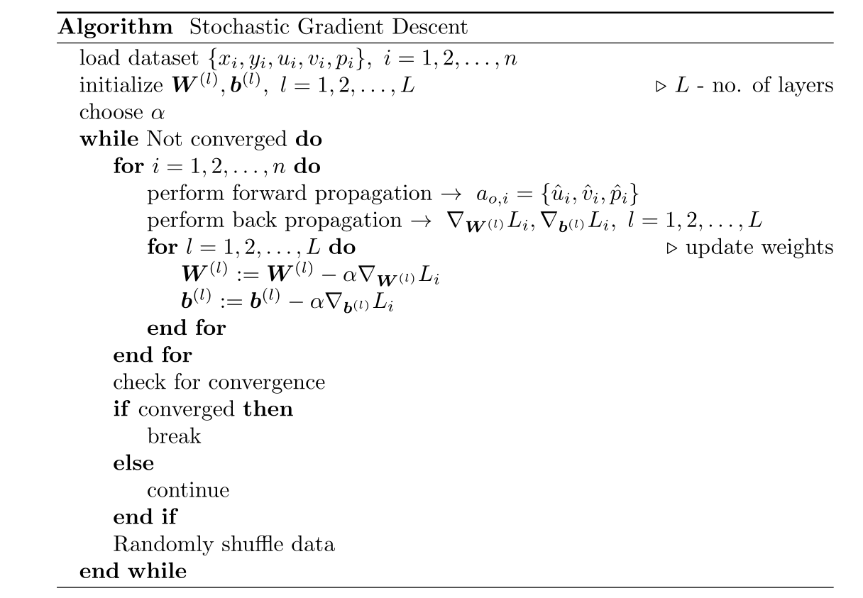
3.5 Optimiziation algorithms - Stochastic Gradient Descent

In this algorithm, the weights will be updated for each record in the dataset

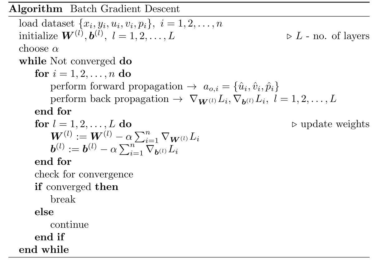
3.6 Optimization algorithms - Batch Gradient Descent

In this algorithm, the weights will be updated after computing gradients for all the records in the dataset

3.7 Optimization algorithms - summary

Batch Gradient Descent
- weights are updated at the end of each iteration with full data
- takes less iterations to converge - as update is performed with all data at once
- used for small datasets

Stochastic Gradient Descent
- weights are updated after each record in the dataset
- memory efficient - stores one step of gradients only
- used for large datasets

Other optimization algorithms that are variants of these two algorithms
- mini-batch gradient descent
- Adaptive gradient (ada grad)
- Adaptive moment estimation (Adam)