1 Abstract
A physics-informed neural network (PINN) is an artificial neural network that learns the function from mathematical constraints that govern the underlying physics to be modelled. In this work, a PINN was built from scratch using the Python programming language with fundamental libraries such as NumPy, pandas, and Matplotlib. The aim of the present work is to develop a fundamental understanding of how a PINN works from both the mathematical and programming points of view. Here, a classical fully connected neural network was constructed and tested by approximating a simple parabola. Further, the built network was developed to be physics-informed and validated by solving the ODE governing the exponential velocity decay of a fluid due to viscosity. The understanding gained will be extended in further scientific computing applications using neural networks.
2 Introduction to neural networks
Machine learning is a branch of mathematics and computer science that develops mathematical models that learn and mimic human behavior. Deep learning is a subset of machine learning that deals with artificial neural networks.
A neuron is a mathematical function that takes in multiple weighted inputs and returns a single output. It is similar to a biological neuron in terms of connectivity and activation. Mathematically, it is represented as below.
f_{neuron} = \sigma\left( \mathbf{w}^T \cdot \mathbf{x} + b\right)
Here, \mathbf{x} is the input vector to the neuron and \mathbf{w} is its corresponding weights vector. b is the bias of the neuron and \sigma is the activation function.
A neural network is a set of interconnected, mathematically modelled neurons that can work as a function approximator. It is based on the universal approximation theorem (Cybenko 1989), which states that any mathematically represented function f(x) can be approximated by a neural network G(x) of sufficient width and depth, to a tolerance \epsilon. Mathematically,
| G(x) - f(x) | < \epsilon
Today, neural networks are of many types, but the fundamental ones are of three kinds: fully connected networks, convolutional neural networks, and recurrent neural networks, each serving a specific purpose. A fully connected network, also called a dense network, is a set of layers of neurons in which each neuron in each layer is connected to all other neurons in nearby layers. These are good at approximating functions that involve scalar input/output variables. Convolutional neural networks are best suited for field-data inputs and outputs, while recurrent networks are suitable for sequential data.
In the present work, a fully connected neural network is developed from scratch and later turned into a physics-informed network. The mathematical background and the problems solved with the developed network are discussed in the sections that follow.
3 Mathematical view on network training
Consider the example network shown in Figure 1. Here, the input data x is fed to a fully connected network that estimates the output data \hat{y}, which is then compared with the expected output data y through a loss function.
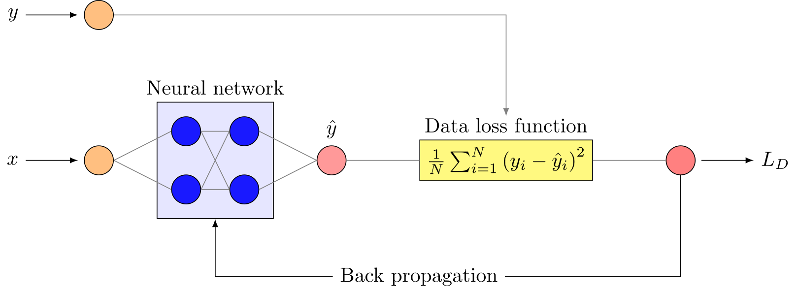
The weights and biases of the example network are then optimized with the loss as the objective function, minimizing it to match the expected output values through an algorithm called backpropagation. The main reference for these backpropagation equations for a fully connected network is (Deriving the Backpropagation Equations from Scratch (Part 1), n.d.).
Mathematically, a single layer l is represented as given below.
\mathbf{x}^{[l]} = \sigma\left( \mathbf{z}^{[l]}\right)
where,
\mathbf{z}^{[l]} = \mathbf{W}^{[l]}\cdot\mathbf{x}^{[l-1]} + \mathbf{b}^{[l]}
Here, \mathbf{W}^{[l]} is the weight matrix and \mathbf{b}^{[l]} is the bias vector of layer l. \mathbf{x}^{[l-1]} is the activated output of the previous layer l-1, and \sigma is the activation function. Let L be the loss function evaluated at the end of the last layer. Then, the gradient of the loss function with respect to the unactivated output of the last layer, z^{[l]}, is given as below.
\left.\frac{\partial L}{\partial \mathbf{z}^{[l-1]}} = \left[\mathbf{W}^{[l]} \right]^T \cdot \frac{\partial L}{\partial \mathbf{z}^{[l]}} * \frac{\partial \sigma}{\partial \mathbf{z}}\right\vert_{[l-1]} \tag{1}
Equation 1 is called the error of a layer. The error is backpropagated from layer l to the previous layer l-1 by the above equation. Here, * is the element-wise multiplication. To begin this backpropagation, we need the above error derivative \partial L/\partial z for the last layer in the network.
The computation of the error for the last layer involves the differentiation of the loss function L with respect to the estimated output \hat{y}. Let the last layer be described as given below.
\mathbf{\hat{y}} = \sigma\left(\mathbf{z}\right)
And let the loss function be the classical mean squared error, as given below.
L = \frac{1}{N}\sum_{i=1}^{N} \left(\hat{y}_i - y_i\right)^2
Then, the error for the last layer is calculated as shown below.
\left.\frac{\partial L}{\partial \mathbf{z}}\right\vert_{[l]} = \frac{\partial L}{\partial \mathbf{\hat{y}}} \cdot \frac{\partial \mathbf{\hat{y}}}{\partial \mathbf{z}} = \frac{\partial L}{\partial \mathbf{\hat{y}}} \cdot \frac{\partial \sigma}{\partial \mathbf{z}} = \left(\frac{2}{N}\sum_{i=1}^{N}\left(\hat{y}_i - y_i\right)\right) \left.\frac{\partial \sigma}{\partial \mathbf{z}}\right\vert_{[l]}
The above equation completes the error computation for all the layers. Next, we must compute the derivatives of the loss with respect to the weights and biases of all the layers using these error vectors. The gradients of the loss with respect to the weights and biases are computed using the error vector for each layer, as shown below.
\frac{\partial L}{\partial \mathbf{W}^{[l]}} = \frac{\partial L}{\partial \mathbf{z}^{[l]}} \cdot \left[\mathbf{x}^{[l-1]}\right]^T \tag{2}
\frac{\partial L}{\partial \mathbf{b}^{[l]}} = \frac{\partial L}{\partial \mathbf{z}^{[l]}} \tag{3}
So, with the above gradient equations Equation 1, Equation 2, and Equation 3, the weights and biases of all the layers can be computed and optimized with the aim of minimizing the loss function. An example problem with a data-driven network is given below, solved with the neural network built using the above equations.
4 Validating neural network code
A couple of datasets were chosen for validating the developed neural network code. The first is a simple parabola curve that the network has to approximate, and the second is a normalized flight velocity profile that the network code also has to approximate. Each problem is explained in detail below.
4.1 Parabola problem
The problem was framed as approximating the parabola curve defined by the equation y = x^2 with x \in [0,0.5].
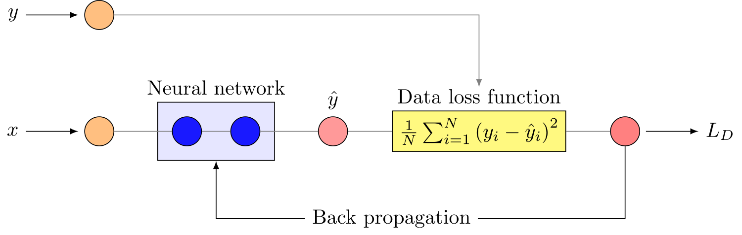
A network with three layers and a single neuron on each layer, i.e., two hidden layers and one output layer, was built for this problem. \tanh() is used as the activation function for all layers, and mean squared error (mse) is used as the loss function for the network. The schematic of the network for this problem is given in Figure 2.
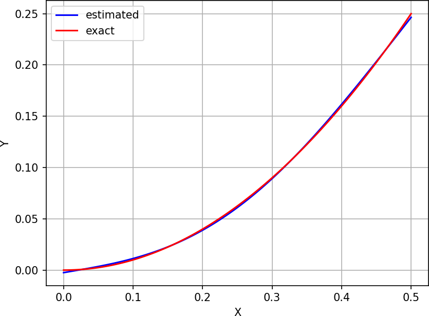
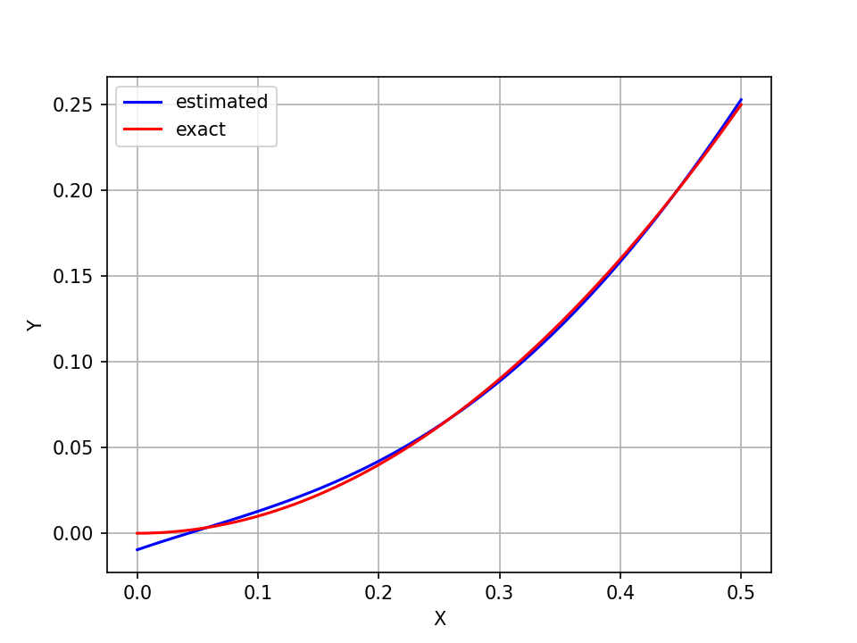
Training was performed on the generated data, and the resulting estimated vs. exact profiles are shown in Figure 3. It can be seen that the estimated result is accurate enough to approximate the y=x^2 equation within the range x,y \in [0,0.5]. Accuracy analysis was not performed, as the goal was to check whether the network code works.
4.2 Flight velocity profile
The second validation was performed using a flight velocity profile obtained from a flight dynamics simulation done for an academic assignment. The profile was smooth and had both positive and negative curvature, hence it was chosen for this work.
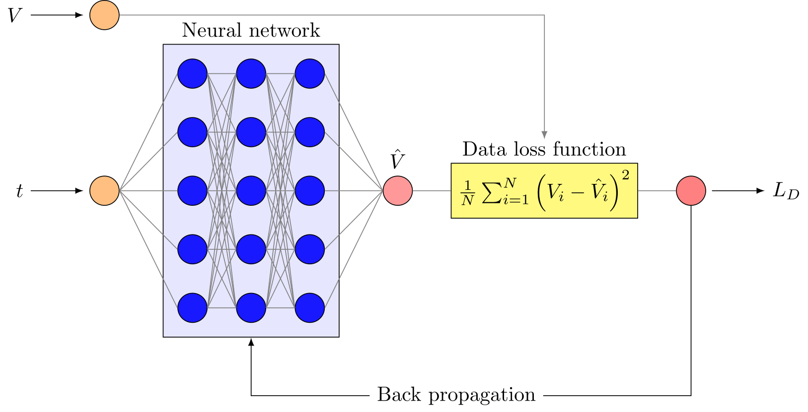
The schematic of the neural network built for this approximation is shown in Figure 4. The network has 5 neurons across 3 hidden layers and 1 neuron for the output. The same \tanh() activation function was used in all layers.
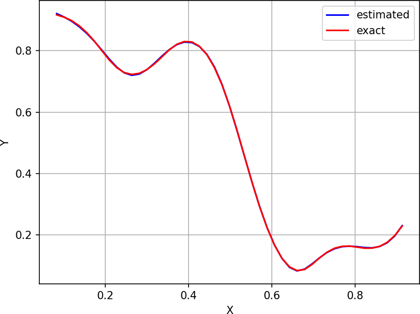
The estimated vs. exact flight velocity profiles are given in Figure 5. It can be seen that the estimate matches the exact velocity profile quite well, proving that the network code is correct. The next step, enhancing the code to include physics information, was therefore carried out.
5 Enhancing the network with physics information
The already developed neural network code was validated against two datasets, and the code now had to be enhanced to include physics information in the form of mathematical constraints.
For each problem to be solved with this network code, the code had to be modified to include the mathematical constraints in the last layer or so. The mathematical constraints can be of two types: algebraic or differential equations. Algebraic equations involving output and input variables can be coded directly, but coding differential equations requires the derivatives to be computed using automatic differentiation in the network, which was accomplished as explained below.
5.1 Computing derivatives of output with respect to input
Differential equations (ODEs and PDEs) involve the derivatives of dependent variables with respect to independent variables. In network terms, the dependent variables are the output variables, and the independent ones are the input variables. Thus, similar to the loss derivative equations, an equation for computing the derivative of a layer’s output with respect to its input was derived.
Keeping the backpropagation equations as the base idea, the matrix equation for \partial \sigma/\partial x of a layer was properly derived and is given below.
\left[\frac{\partial \sigma}{\partial \mathbf{x}}\right] = \left[\mathbf{W}\right]^T \cdot \text{diag}\left(\frac{\partial \sigma}{\partial \mathbf{z}}\right) \tag{4}
Here, \partial \sigma/\partial x is a vector of the layer, and \text{diag}\left(\partial \sigma/\partial x\right) is a diagonal matrix with those vector elements on the diagonal. \left[\frac{\partial \sigma}{\partial \mathbf{x}}\right] is a matrix of the same size as \left[\mathbf{W}\right]^T.
It should be noted that Equation 4 gives the derivative of the output with respect to the input of a single layer only. The chain rule in differential calculus must be used to obtain the derivative of the overall network output with respect to its actual input.
5.2 Validating the gradient equation
The matrix equation in Equation 4 was validated by testing it on a network trained on pure data. A network was built and trained using synthetic data of fluid velocity decay at a point in the flow due to fluid viscosity. The synthetic data was generated using the equation below with k = 5.0 and V_0 = 1.
V(t) = V_0 e^{-k t}
And its corresponding ODE for derivative computation is given below.
\frac{d V}{d t} = -k V
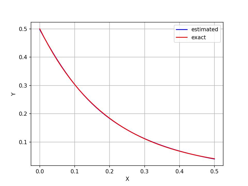
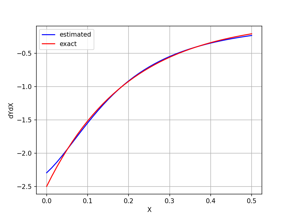
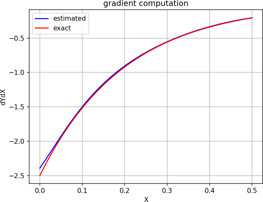
The network was trained for X = t = [0,0.5] and the corresponding velocity values. The estimated vs. exact velocity decay profile is given in Figure 6 (a). The trained layer weights were then used to compute the derivative dV/dt, which was compared to the exact values and is given in Figure 6 (b). It can be seen that the derivative profiles match quite well, except at the beginning, which is due to a limitation in approximating the velocity profile — a limitation that was later rectified when validating the PINN network. Thus, the derivative computation is validated, and the next step was to validate the self-built physics-informed neural network.
6 Validating the Physics-Informed Neural Network (PINN) code
Validating the enhanced PINN code was done with two chosen problems. The first is to approximate the same parabola profile, but using the equation y=x^2 instead of y-data, and the second is to model the fluid velocity decay profile due to fluid viscosity, which involves a differential equation.
6.1 Parabola profile with equation
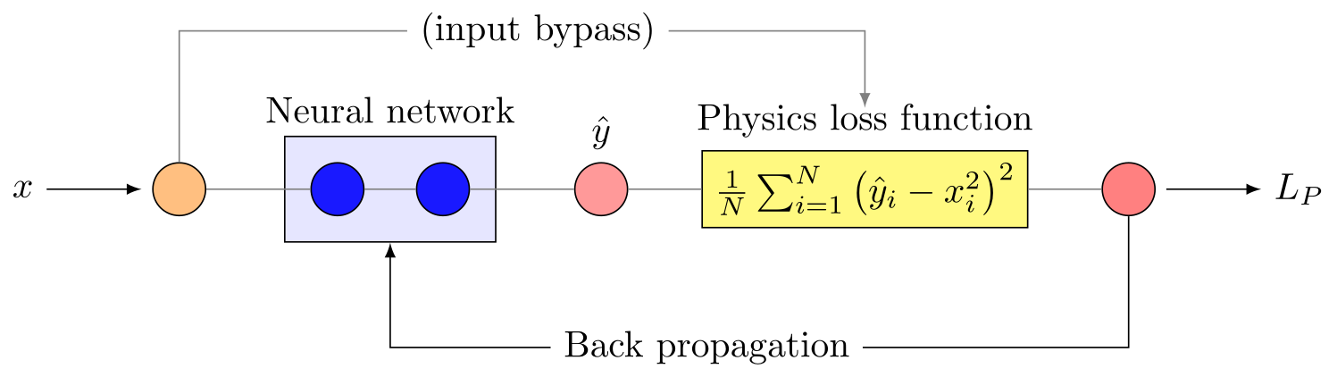
This problem is similar to the one used for validating the neural network code earlier, except that the y-data is made unavailable and the governing equation y=x^2 is given instead. The residual of the equation is fed to the loss function, which has to be minimized to train the model. The network architecture is given in Figure 7, and the estimated vs. expected results are given in Figure 8.
6.2 Exponential velocity decay due to fluid viscosity
Given a point in a free fluid flow, the velocity of fluid particles at that point decays due to the resistance termed fluid viscosity. This decay is exponential in form and is governed by Equation 5, which was already discussed partially in the derivative validation section.
\frac{d V}{d t} = -k V \tag{5}
Here, k is a constant denoting fluid viscosity. The equation is autonomous and has the analytical solution given below.
V = V_0 e^{-k t}
V_0 is the initial velocity of the fluid flow. A schematic of the PINN used for the problem is given in Figure 9. Here, the network has two hidden layers with 3 and 2 neurons respectively, and an output layer with 1 neuron. The \tanh() activation function was used in all layers.
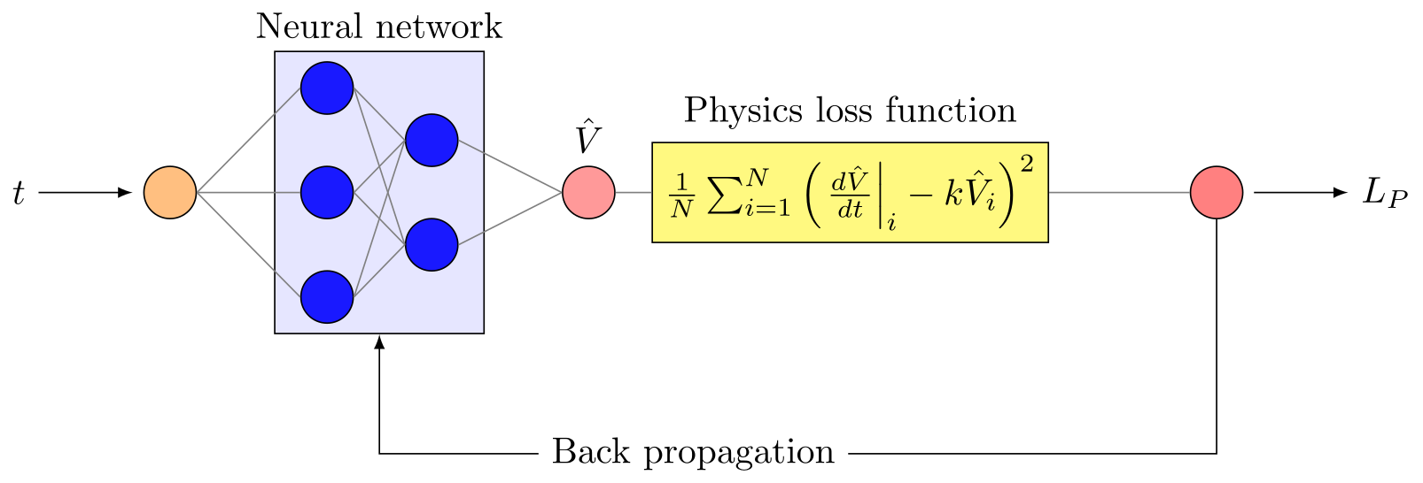
The loss function of this network is made up of two parts. The first part enforces the initial condition on velocity and is active only at the start of the time data; it is given below.
L_{IC} = \left.\left(\hat{V}_i - V_i\right)^2\right|_{t=0, i=0} \tag{6}
The second part contains the governing-equation constraint and is executed for all timesteps. The equation is given below.
L_{ODE} = \frac{1}{N}\sum_{i=0}^{N}\left(\left.\frac{d\hat{V}}{dt}\right\vert_i - k\hat{V}_i\right)^2 \tag{7}
So, the total loss function for the network is the sum of Equation 6 and Equation 7, as given below.
L = L_{IC}+L_{ODE} = \left.\left(\hat{V}_i - V_i\right)^2\right|_{t=0, i=0}+\frac{1}{N}\sum_{i=0}^{N}\left(\left.\frac{d\hat{V}}{dt}\right\vert_i - k\hat{V}_i\right)^2 \tag{8}
To increase the weighting of the initial condition, since it is active only in a part of the backpropagation, a factor of 10 was applied to its component, and the final loss equation is given below.
L = L_{IC} \times 10+L_{ODE} \tag{9}
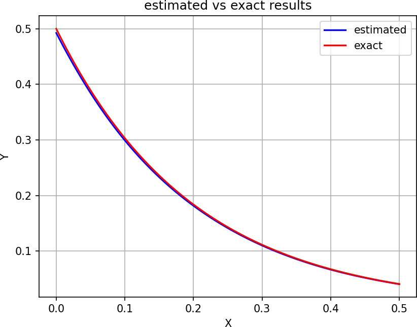
The model was trained successfully, and the estimated results for the velocity profile and the derivative computation are given in Figure 10. It was found that the estimated derivative was more accurate than the one shown in the validation section. This is because a network that learns a function through physics constraints learns better than one that maps the same function purely through data.
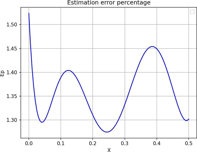
The error percentage graph for the estimated vs. expected velocity profiles is given in Figure 11. The error percentage was in the order of 1–2%, which validates the PINN code developed.
7 Python code structure
Each source code package provided in the github repo contains three Python scripts, each handling a specific part of the program. They are listed below.
script_main.pyinputData.pycustomLayers.py
script_main.py is the main script that constructs the network and contains the snippets related to physics information. inputData.py contains the snippets that determine the input parameters, such as the number of layers and neurons per layer, whether to save/load weights, and the learning-rate adaptation code. Finally, customLayers.py contains the class definition of a neural network layer, which holds everything related to a layer, such as its activation function, its derivative, and its forward evaluation. The activation function is currently hard-coded, and may be made generalizable later.
The code was made generalizable in terms of the number of neurons/layers, and is written for a fully connected dense network. Future work may include custom code for other network types as the need arises.
8 Conclusion and future work
I conclude the present work by stating that a high level of understanding and knowledge was gained from the mathematical and programming perspectives of neural networks, which opened gateways to other methods of using neural networks, such as optimizing the input values themselves based on loss to find optimal values, and so on. The present work is limited to the generalized code for a fully connected dense network. This code may be extended for other scientific computing applications, such as Neural ODEs.
9 Acknowledgement
The mathematical foundations of neural networks were taught expertly by my professor, Dr. Sumitra S., Department of Mathematics, Indian Institute of Space Science and Technology. I am deeply grateful to her for the Graphical Models and Deep Learning course, without which this work would not have been possible.