Content
Conceptual Example and introduction
PSO algorithm and its mathematics
Advantages, limitations and variants
Assignment problem
References
Lecture
Multi-disciplinary Design Optimization
by
Department of Aerospace Engineering,
Indian Institute of Space science and Technology,
Thiruvananthapuram, Kerala - 695547
2026-03-24
Conceptual Example and introduction
PSO algorithm and its mathematics
Advantages, limitations and variants
Assignment problem
References
Himmelblau function
\[ f(x,y) = \left(x^2+y-11\right)^2+\left(x+y^2-7\right)^2 \]
Swarm intelligence-based meta-heuristic evolutionary algorithm. It is inspired from the nature, like a flock of birds, a school of fish etc…
Introduced by Kennedy and Eberhart in 1995 [1]
Swarm intelligence: the particles are not only communitcate with one another, they also influence one another’s behavior and equipped with a memory-like feature to keep track of best position it encountered thus far
Meta-heuristic: A strategy that guides the search process, rather than directly solving the problem
Each particle will carry two aspiration points: the best point visited by the swarm thus far, and the best point previously encountered by the said particle.
This enables to reach optimum solution much quicker than non-swarm intelligence-based, population based algorithms like the genetic algorithm.
PSO’s computational algorithm is based on simple and primitive vector-based mathematics only.
It is a parallelizable, gradient-free algorithm with less memory requirements and is independent of problem type: linear/non-linear, continuous/discrete etc…
It can yield a fast, global and mostly suboptimal solution to the given problem
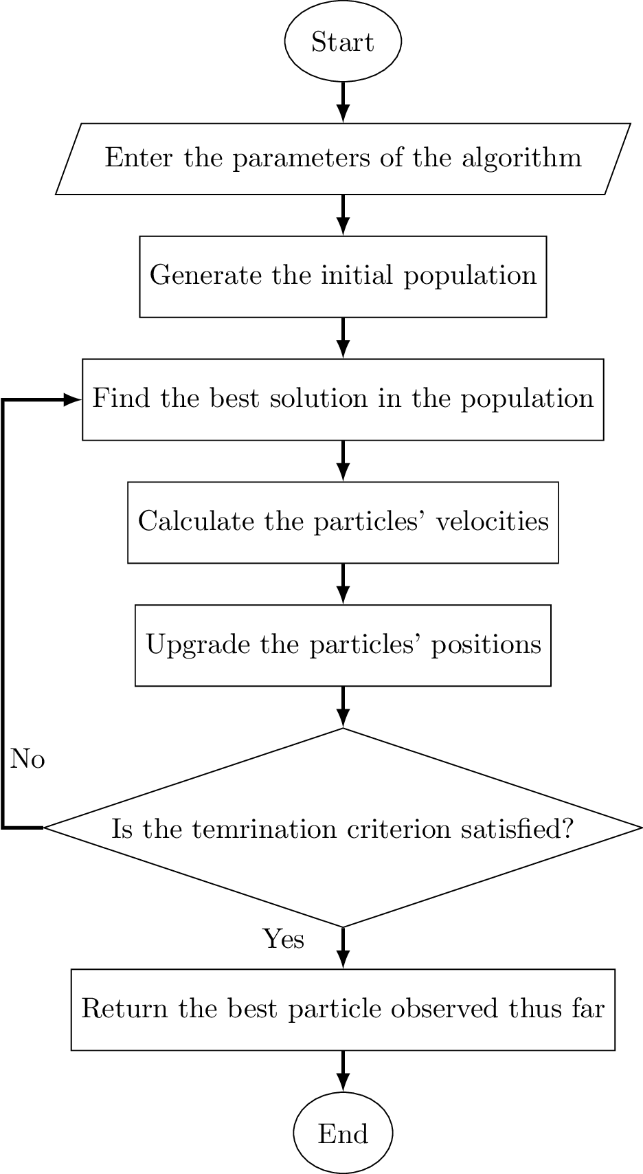
There are three stages
Initialization stage
Searching stage
Termination stage
Let, \(N\) - number of dimensions in the design space
Let, \(X\) - denotes a particle array
\[ \begin{aligned} X = \begin{bmatrix} x_1 & x_2 & \dots & x_N \end{bmatrix} \end{aligned} \]
Let, \(M\) - denotes population size i.e. number of particles. And let \(pop\) denotes the population, then
\[ \begin{aligned} pop = \begin{bmatrix} X_1 \\ X_2 \\ \vdots \\ X_M \end{bmatrix} = \begin{bmatrix} x_{1,1} & x_{1,2} & \dots & x_{1,j} & \dots & x_{1,N} \\ x_{2,1} & x_{2,2} & \dots & x_{2,j} & \dots & x_{2,N} \\ & & & \vdots & \\ x_{i,1} & x_{i,2} & \dots & x_{i,j} & \dots & x_{i,N} \\ & & & \vdots & \\ x_{M,1} & x_{M,2} & \dots & x_{M,j} & \dots & x_{M,N} \\ \end{bmatrix}_{M\times N} \end{aligned} \]
All \(x_{i,j}\) are randomly initialized
\(P_{best}\) - best position found by the particle
\[ \begin{aligned} P_{best,i} = \begin{bmatrix} p_{i,1} & p_{i,2} & \dots & p_{i,N} \end{bmatrix} \ \ \ \forall i \end{aligned} \]
\(G_{best}\) - best position found globally by the swarm
\[ \begin{aligned} G_{best} = \begin{bmatrix} g_{1} & g_{2} & \dots & g_{N} \end{bmatrix} \end{aligned} \]
Initially, \[ \begin{aligned} \mathbf{P}_{best} = \begin{bmatrix} P_{best,1} \\ P_{best,2} \\ \vdots \\ P_{best,M} \end{bmatrix}_{M\times N} = pop \end{aligned} \]
The idea behind the PSO algorithm is to coordinate the motions of the particles as they enumerate the search space
The motion of each particle is captured by its velocity vector \(V_i\)
\[ \begin{aligned} V_i = \begin{bmatrix} v_{i,1} & v_{i,2} & \dots & v_{i,N} \end{bmatrix} \ \ \ \forall i \end{aligned} \]
The velocity of each particle along each dimension in design space has to be updated during every iteration using
\[ v_{i,j}^{new} = \omega \times v_{i,j} + C_1 \times r_1 \times \left(p_{i,j} - x_{i,j}\right) + C_2 \times r_2 \times \left(g_j - x_{i,j}\right) \ \ \forall i,j \]
where
\(C_1, C_2\) are the model parameters of PSO algorithm
\(\omega\) - inertia of each particle, a non-zero positive number is dynamically adjusted by the algorithm to reduce over iterations
\(C_1\) - Cognitive parameter, a non-zero positive number that determines how much weigtage to be given for personal best position found by each particle
\(C_2\) - Social parameter, a non-zero positive number that determines how much weightage to be give for the global best position found by the swarm by each particle
\(r_1,r_2\) - random numbers introducing stochastic nature into the process
After computing new velocitiesm, the position of each particle along each dimension in the design space is updated as
\[ x_{i,j}' = x_{i,j} + v_{i,j}^{new} \ \ \ \forall i,j \]
\[ \begin{aligned} X_{i,j}^{new} = \begin{bmatrix} x'_{i,1} & x_{i,2}' & \dots & x_{i,N}' \end{bmatrix} \ \ \ \forall i \end{aligned} \]
There is no explicitly defined, unique termination mechanism
Some mechanisms from literature are
Another mechanism to make the algorithm to stop is the Inertia reduction
Inertia \(\omega\) is popularly reduced in two ways
Linear method \[ \omega_t = \omega_0 - \left[\left(\omega_T - \omega_0\right)\times\frac{t}{T}\right] \ \ \ \forall t \]
where \(\omega_0\) and \(\omega_T\) are the initial and final user-defined inertia values
Geometric method \[ \omega_t = \omega_0 \times \gamma^t \ \ \ \forall t, \ \ \ \gamma \in (0,1) \]
Define the objective function \(f_{obj}(.)\)
Define number of particles in the swarm \(M\)
Define the termination criterion
Define the initial inertia of particles \(\omega_0\), Cognitive parameter \(C_1\) and Social parameter \(C_2\)
Initialize the particle positions randomly and uniformly in the design space
Compute the \(P_{best}\) and \(G_{best}\) arrays by evaluating the \(f_{obj}(.)\) over all the particles’ positions
Compute the velocity vector of each particle with updated \(P_{best}\) and \(G_{best}\)
Update the position of each particle with computed velocity
Repeat steps 6, 7 and 8 until the termination criterion is satisfied
Return the \(G_{best}\) array as the final design variable values.

There are many variants of PSO algorithm from the literature, some of them are
PSO is applied in almost all of the scientific fields, some examples are
Main reference
The main reference for this algorithm is: [8]
Take one of the functions from here
Develop a computer program, with any programming language, applying the PSO algorithm on to the chosen function
Create a brief report with results and computer program, and submit to ramkumars.24@res.iist.ac.in
![]()
Particle Swarm Optimization